2 layers135.1 × 159.4 mm

 fl4p/dcdc-parasitics
KiCad → FastHenry extractor for half-bridge power-stage parasitics (commutation-loop L, common-source inductance, gate-loop L/R) → SPICE subckt + SVG schematic
ReboostV2.1 fixed is an open-source printed circuit board by fl4p, from the fl4p/dcdc-parasitics repository on GitHub. It is a 4-layer board of 94.5 × 80.5 mm with 184 parts on 113 nets, routed with 1,436 tracks and 278 vias.
It is built around the 74LVC2G08, LTC6362IDD and CP2104-F03-GM, with the LTC3639EMSE#PBF, ISO1044 and LP2985AIM5-3.3 among its other parts. Its parts include 70 capacitors, 56 resistors, 13 diodes, 12 ICs and 8 inductors. It belongs with the interfaces and adapters boards and the STM32 boards of this library.


Extracts the half-bridge power-stage parasitic inductances and resistances from a KiCad PCB for:
You give it the switch-node net and the GND net; everything else (HS/LS FETs, Vin rail, gate nets, input caps) is auto-discovered from connectivity, with overrides for every guess.
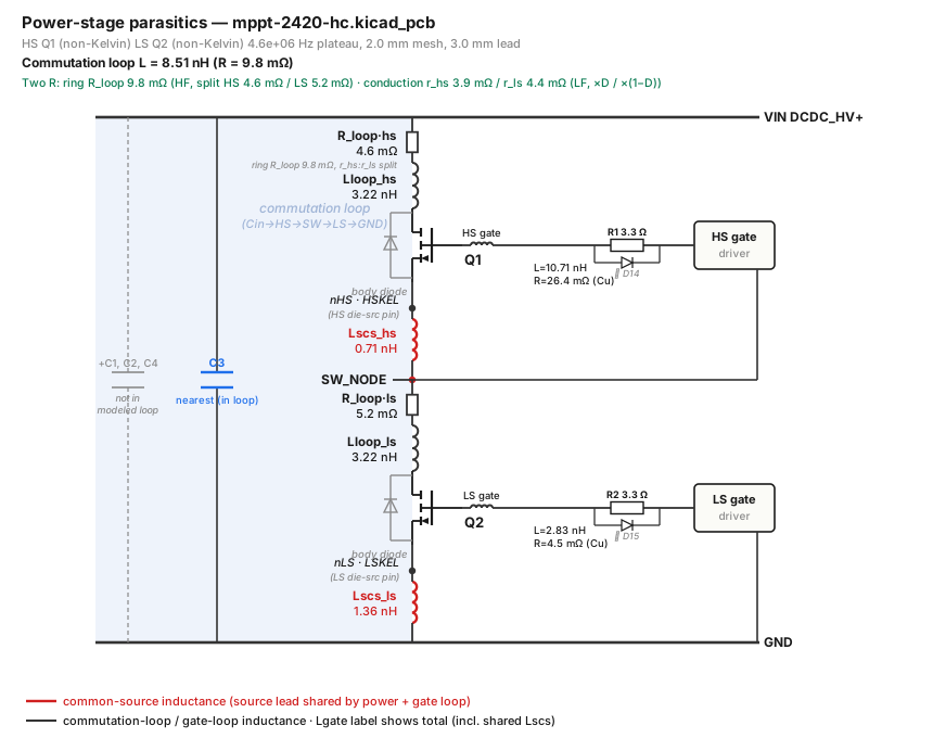
Half-bridge parasitics extracted from the open-hardware
LibreSolar MPPT 2420 HC (4-layer
synchronous buck), rendered by --svg: each parasitic as a labelled coil, the
two common-source source-leads in red, the input-cap bank (the ported cap and
the greyed-out ones), and the auto-detected gate network (Rg). This is the
historical lead-inclusive fixture and is retained as an output-format showcase;
its numeric labels are not a current copper-only validation.
Each extraction basis uses one FastHenry solve with multiple ports to obtain its
full mutual-inductance matrix. The baseline/full-loop extraction and the
lead_mm=0 identity-matrix path need one solve. A non-identity matrix Cin request
may run three matched bases (full_loop, cap_only, and switch_residual) so
the producer can separate cap-side and switch-side copper without mixing gauges.
| Port | Across | Gives |
|---|---|---|
P_pwr | nearest Cin — MLCC (Vin ↔ GND) | commutation-loop L, HF ring R |
P_ghs | HS gate driver-end ↔ HS gate return | HS gate-loop L |
P_gls | LS gate driver-end ↔ LS gate return | LS gate-loop L |
P_bulk | nearest bulk electrolytic (Vin ↔ GND) | LF conduction-loop R |
P_hs | Vin(bulk) → SW, via HS leads | HS conduction R |
P_ls | SW → GND(bulk), via LS leads | LS conduction R |
P_probe_<name> | any declared REF.PAD ↔ REF.PAD (opt-in, see probe_ports) | mount-loop L/R of that position |
Palace is the primary maintained electrostatic solver. The
palace-electrostatic-pcb-gates-v2 path uses conformal tetrahedral volume
meshes, finite closed conductor terminals, explicit air/dielectric material
volumes, and a declared outer Dirichlet boundary that approximates
electrostatic infinity. That boundary is never treated as PE, chassis, a PCB
net, or SPICE node 0; an outer-domain expansion ladder is mandatory.
lib/palace_mesh.py writes the qualified Gmsh fixtures. Real PCB geometry uses
lib/palace_plc_mesh.py: MeshPy nodes one global planar conductor/material
arrangement, that exact arrangement is reused at every geometry z-plane, and
triangular prisms receive a deterministic conformal tetrahedral split. It
rejects open/non-manifold shells, incomplete terminal/material coverage, and
nonpositive tetrahedral Jacobians, then emits first-order Gmsh 2.2 directly.
lib/palace_build.py binds the pinned source patch, CMake caches,
linked libraries, launcher, wrapper, and binary. lib/palace.py binds those
manifests to Palace JSON configs, runs the solver, gates an independently
ordered 17-digit terminal reaction-charge Maxwell matrix against Palace's
energy matrix, and preserves exact streams, resolved config, runtime metadata,
and execution identity. The qualification build also hard-checks explicit
||b-Ax||/||b|| after every terminal solve. Mesh,
polynomial-order, and finite-domain ladders over the frozen air, enclosed-FR4,
and PCB-like fixtures must pass before any Fugu run. See
docs/palace-electrostatic-qualification-plan.md.
Production launches use a content-addressed user-space execution snapshot whose config, mesh, launcher, solver, and helper bytes are validated before and after the process. Ordinary runs select a bounded local resource class. Checkpointed runs additionally require a finite resource decision and a canonical E5 ledger attempt before launch; every attempt receives a fresh snapshot/output root, and matrices are consumable only through the terminal ledger capability.
The complete 24-rung fixture ladder has passed. extract_palace_mesh.py runs
the two-interpreter KiCad adapter, preserves every named net and flashed no-net
item separately, retains NPTH holes as voids rather than terminals, and binds
PCB, dump, stackup/material policy, geometry controls, mesher, and output bytes:
PYTHONPATH=out/palace-qualification/venv/lib/python3.14/site-packages \
  python3 extract_palace_mesh.py board.kicad_pcb \
  --material 'Top Solder Mask=3.3' \
  --material 'Bottom Solder Mask=3.3' \
  -o out/palace-pcb-geometry
Material overrides are explicit assumptions, not validated values. A physical Fugu model still requires source-bound P2 evidence, convergence ladders, independent review, and actual material identification or bounded sensitivity.
lib/fastercap.py provides the independent 3-D electrostatic path: it closes
conforming 2-D triangle meshes into finite-thickness conductor surfaces, emits
closed interfaces between dielectric regions, writes self-contained FasterCap
panel files, and runs the headless solver through $FASTERCAP. Each deck has a
hashed sidecar manifest with stable solver labels. The runner returns a Maxwell
matrix only after exact label identity, normal termination, final automatic-norm,
per-RHS GMRES, live process-tree resource, raw reciprocity/passivity, strict
post-average passivity, and exact branch-reconstruction gates pass. Complete
matrices from failed or partial runs remain diagnostic-only. Manual fixed--m/
fixed--t probes use a separate API and never expose a qualified matrix. The
backend-neutral lib/maxwell.py validates matrix symmetry/passivity, converts
Q = C_M V into pairwise plus reference capacitors, reconstructs the original
matrix for an exact contract check, and emits a passive SPICE subcircuit. The
runner enforces a separate per-coupling reciprocity tolerance before returning
the symmetric average; FasterCap's -a tolerance controls refinement
convergence and is not reused as a reciprocity bound. Every invocation preserves
byte-exact content-addressed stdout/stderr and writes either a
rejected_diagnostic manifest or a numerically_converged_diagnostic manifest
under gate policy fastercap-pcb-gates-v1. Diagnostic convergence is not a
physical-model qualification.
This foundation is deliberately not wired into extract_parasitics.py yet.
extract_capacitance.py provides the first two-interpreter KiCad adapter: a
stdlib-only KiCad Python step dumps exact filled-zone contours in millimetres,
then system Python uses Shapely 2.1 constrained triangulation to close grouped
copper surfaces and converts every panel coordinate to FasterCap SI metres. For
example:
python3 extract_capacitance.py board.kicad_pcb \
  --group SWITCH=SW --group RETURN=PGND,GND \
  -o out/electrostatic-geometry

# Explicit opt-in reduced diagnostic representation
python3 extract_capacitance.py board.kicad_pcb \
  --group SWITCH=SW --group RETURN=PGND,GND \
  --representation effective-thickness \
  --effective-thickness-um 34 --anchor midplane \
  -o out/electrostatic-geometry-reduced
Generated names encode source, representation, material scope, and lifecycle,
for example filled_zones_physical_air_only_diagnostic.lst and
filled_zones_effective_34um_midplane_air_only_diagnostic.lst. Geometry metadata
uses a canonical content hash in its filename. Its fail-closed loader verifies
the filename/content ID plus the referenced deck, deck manifest, and reduction
provenance hashes. The deck manifest binds the same reduction provenance and its
hash; solver run manifests then bind the deck manifest plus all solver settings
and streams.
Both decks are geometry-development diagnostics, not physical PCB capacitance
models. They exclude tracks, pads, vias, and copper graphics and do not yet emit
the parsed stackup's dielectric interfaces. The only fixture-qualified reduction
is watertight closed 35 µm to 34 µm copper, midplane anchored, for overlapping
1 mm square parallel plates in air with a 100 µm source face gap and an explicit
pinned synthetic-fixture context. The reusable API marks any PCB/Fugu2 or
full-stackup use outside_fixture_envelope, fixes
physical_validation_authorized=false, and caps its lifecycle at
numerically_converged_diagnostic.
The content-addressed geometry manifest records limitations, PCB and contour-dump
hashes, KiCad version/interpreter, dump record count, areas, repair counts,
simplification error, minimum boundary segment, triangle/panel counts, source and
effective thicknesses, anchor, gap/displacement errors, qualification scope, and
artifact class. Use --geometry-tolerance (mm, default 0.001) as an explicit
panel-convergence knob; geometry that exceeds the area-error gate is rejected.
Start solver validation with the synthetic fixture:
python3 examples/fastercap_parallel_plate.py -o out/fastercap-parallel-plate
FASTERCAP=/path/to/FasterCap \
  python3 examples/fastercap_parallel_plate.py --run \
  -o out/fastercap-parallel-plate
The first command only emits inspectable geometry. The second writes
capacitance.lib only when every fastercap-pcb-gates-v1 solver and matrix gate
passes. Unpatched FasterCap 6.0.7 macOS builds may emit
Error: cannot retrieve the information about the free memory quantity; the
fail-closed runner preserves a rejected_diagnostic manifest and returns no
matrix for those builds. The local macOS build uses Mach VM statistics for this
resource check and passes the real parallel-plate smoke test. See
docs/fastercap-slice1-diagnosis.md. A solver build that terminates without
diagnostics additionally reports plate-to-plate capacitance against the ideal
estimate; fringing means the ratio is not exactly one.
In the full-loop basis, both FET channels are shorted at the die plane
(.equiv drain_die source_die)
and each gate is closed to its source there, so P_pwr traces the full
Cin → HS → SW → LS → GND → Cin shoot-through loop and each gate loop shares that
FET's source lead. CSI then falls out as the side-specific mutual
M(P_hs, P_ghs) / M(P_ls, P_gls) — the shared source-lead partial inductance
that the gate driver actually sees. The older full-loop mutual is still recorded
as csi_hs_loop / csi_ls_loop in JSON for diagnostics. Whether the gate return
taps the die-source (Kelvin, CSI excluded) or the power-source pad
(non-Kelvin, full CSI) is encoded by where the gate-return node is placed
(default: non-Kelvin / worst case; force with --hs-kelvin / --ls-kelvin).
--cin-parallel N)By default P_pwr sits across the single nearest ceramic, which ignores the
other input caps that share the commutation current. For a pure-inductance port
matrix the parallel loop L is then lower than the single-cap number, so it usually
over-estimates SW-node overshoot -- but that is not a bound on the extracted
complex Z: copper R can put the parallel value above the single cap (see the two
references below). --cin-parallel N ports the N nearest input ceramics in the same
solve, so FastHenry returns their full mutual matrix, and the reduce step forms the
true effective 2-terminal commutation impedance under a common-voltage drive
(every cap pad pair at the same SW-node voltage, gates open):
Z_eff = 1 / (1ᵀ Zc⁻¹ 1) (Zc = N×N cap-port submatrix)which folds in every branch-to-branch mutual Mᵢⱼ exactly (not a naive 1/ΣLᵢ),
solved as Zc x = 1 (never an explicit inverse; cond(Zc) is reported and a
warning fires if it is ill-conditioned). The parallel-cap current split
y = Zc⁻¹·1 is reported per refdes.
The SW-peak loop L comes with two reference values. They are not bounds:
| field | meaning |
|---|---|
L_loop_single | nearest single cap alone |
L_loop_ideal | all N caps ‖, treated as ideal shorts (copper only) |
L_loop_physical | plateau-band result with the uniform per-cap series ESL/ESR supplied by --cin-esl/--cin-esr |
For a pure-inductance matrix, adding cap ESL can only raise the parallel L above
L_loop_ideal, and the parallel never exceeds the best single cap. Neither holds as a
bound on the extracted complex Z: copper R can lift the ideal-cap reduction above
L_loop_single (and the nearest cap need not have the lowest self-L), so treat the two as
references. Use L_loop_physical when cap ESL/ESR are known. L_loop_physical and the top-level current_split are evaluated at the selected
L plateau (default 5 MHz), not at --ring-freq. The reducer applies the same series
ESL/ESR at every point in L_eff_sweep, so that array contains the full effective
loop L/R sweep, including the point nearest the ring. It does not currently emit a
per-cap ring-frequency current split. The series-only cap term is a useful
above-SRF diagnostic; it is not a full C/ESR/ESL capacitor model. The loss tool
supplies that full model from dslib.
Without --cin-esl/--cin-esr the headline remains the ideal-cap copper-only
value. The two references always land in the report/JSON; L_loop_physical is set
only when a series ESL or ESR was supplied. Port polarity is fixed (always
Vin→GND) so a reversed cap cannot silently corrupt the mutuals; a spuriously-low
effective L still trips a warning.
Cap selection. Default is nearest-by-centroid-distance (deterministic, shown in
the manifest as cin_select); bulk electrolytics are excluded by package/type
(THT can/radial, CP_/Elec/tantalum/polymer footprints) — above their SRF they
can't source the tens-of-MHz edge. Classification is by footprint, not value, so
a 10–22 µF 1210 MLCC stays in the HF set while a small electrolytic stays out; the
per-refdes class is recorded in cin_class. Keep the bulk caps with
--include-bulk-cin (e.g. a low-frequency ripple-path study). Override selection
entirely with --cin-loop-refs C17 C18 C9 C16. If you request more caps than
exist, it warns and solves with what it found rather than silently clamping.
The loop resistance is not one number, because it carries current at two frequencies that see different copper and different reference caps:
| R | Freq | Anchored on | Used for |
|---|---|---|---|
R_loop (ring) | ~MHz plateau | nearest MLCC (sources the edge) | SW-node ring Q / damping; skin-elevated |
R_hs / R_ls (conduction) | ~DC fundamental | nearest bulk electrolytic | conduction I²R, split per switch |
At the 39 kHz switching fundamental the MLCCs are ~open and carry no conduction
current — the fundamental is sourced and returned by the bulk electrolytics. So
the conduction ports (P_hs/P_ls/P_bulk) anchor on the nearest bulk cap, not the
ceramic, and their R is read at the lowest swept frequency (skin depth ≫ copper
thickness there, i.e. the near-DC conduction value) rather than at the ring plateau.
P_hs drives Vin(bulk) → SW through the HS drain+source leads (the die short routes
it), so its self-R is that switch's true conduction copper; P_ls likewise for
SW → GND. The residual R_loop_cond − R_hs − R_ls is reported as the SW-node
spreading R. In the emitted .SUBCKT, R_loop is a single solved HF ring
resistance; its HS/LS Rser placement is only a damping distribution, split by
the LF R_hs:R_ls proportion. A reconstruction check warns if the per-side
conduction R exceeds the LF loop R (a port-polarity/SW-reference tripwire).
Boards with an all-ceramic input bank fall back to the nearest ceramic for the
conduction anchor (there the ceramics do carry the fundamental); the anchor
refdes and class are recorded in cond_ref.
Both R_loop and R_hs/R_ls are read at a single characteristic frequency (the ring
plateau and near-DC respectively). To get the AC resistance at an arbitrary
frequency, raise the skin sub-mesh (--nwinc/--nhinc > 1); the per-frequency
L_eff_sweep in the JSON then shows R rising across the band as skin/proximity effect
crowds the current.
cin_skin)"Ring plateau" was itself a compromise: the plateau is read at ~5 MHz, roughly a decade below the band the SW ring actually decays in. Measured on Fugu2:
| band | loop R | vs the exported plateau |
|---|---|---|
| 39 kHz (fsw) | 1.41 mΩ | 0.45× |
3.9 MHz (exported R_loop) | 3.13 mΩ | 1.00× |
| 39 MHz (SW ring) | 5.34 mΩ | 1.70× |
| 84 MHz | 5.48 mΩ | 1.75× — saturated |
The rise is sub-√f and saturates above ~20 MHz: once the skin depth falls below the
35 µm foil the current is already confined, so the textbook √f law over-predicts it. L_loop
is flat over the same span (3.20 → 3.16 nH) — only R moves.
A consumer that places a single R therefore damps its ring with the wrong number (the loss
deck was −71 % on the loop R at the ring). So the reduction also fits a series Foster RL
ladder to the swept solve and exports it as cin_skin: a set of (Rₖ, Lₖ) poles that add 0 Ω at
DC and Σ Rₖ at the ring. Consumers place it in series with the commutation leg on top of the
DC-band branch R (cin_matrix.R_dc) and get the whole curve, not two points. On Fugu2 five
poles track R(f) to 1.2 % from 39 kHz to 84 MHz.
The corners are FIXED (log-spaced) and only the pole resistances are solved, by NNLS — so the
fit is deterministic and Rₖ ≥ 0 by construction (a negative pole would be an active element).
--ring-freq sets the band it must be honest at (default 55 MHz) and --skin-poles the pole
count. The ladder is currently emitted only for a valid identity-basis matrix Cin
model (--emit-cin-network --cin-network-model matrix with pad-ideal
--lead-mm 0 extraction). If the selected Cin basis cannot carry the fit, or if
the sweep (--hf-freq) never reaches the ring band, no ladder is emitted and
cin_skin_unavailable_reason says why. The rise is not extrapolated, and "no
ladder" must never be read as "copper is flat".
--emit-cin-network)For the loss tool's Cin ESR / input-ripple model, --emit-cin-network ports the
full input bank (bulk + MLCC) individually (P_cin_<ref>, separate from the
MLCC-only HF-loop selection so L_loop is untouched). --cin-loop-refs selects
the caps used for the headline commutation-loop reduction;
--cin-network-refs independently restricts the full-bank network. The deprecated
--cin-refs spelling is only an alias for --cin-loop-refs.
Choose the copper model explicitly:
| requested model | behavior | intended use |
|---|---|---|
--cin-network-model matrix | Preserves the full coupled-L cap-port matrix and may resolve to cin_model.mode=matrix or matrix_with_sw_coupling. With lead_mm=0, the accepted identity basis keeps all switch-side board-copper L in the matrix and emits L_sw_element=0 by construction. | Production loss flow; required for heterogeneous banks such as the complete seven-cap Fugu2 bank. |
--cin-network-model scalar_trunk | Legacy reduction to one shared Vin/GND trunk plus one private branch per cap: L[i,i] = L_shared + Lb_i, L[i,j] ≈ L_shared. | Compatibility and homogeneous-bank diagnostics only. |
The scalar reduction emits cin_branches and
cin_L_shared/cin_R_shared; its _raw counterparts preserve the unclamped
diagnostic decomposition. This topology cannot represent every passive coupled
matrix. The extractor therefore validates it and fails closed when it is invalid.
--allow-scalar-cin is an expert override that emits the legacy clamped model; it
does not make the approximation accurate. Consumers must dispatch on
cin_model.mode and cin_model_valid, not blindly consume the scalar fields.
Matrix mode emits cin_matrix, including its basis, cap refs, coupled L matrix,
R_100k, R_dc, realizability metadata, switch-copper ownership, and any resolved
switch coupling. The loss tool normally assembles the Cin SPICE text in memory and
includes the model/provenance header. If that text is instead supplied through a
persisted cin_network.lib, the reader uses its header to refuse stale, invalid,
or undispatchable networks; the extractor itself does not write this .lib.
Both models are copper only — parasitics stays parts-DB-free. The loss tool
enriches each ref with its datasheet C/ESR/ESL from dslib and builds the complete
cin_network. Copper branch resistance is distinct from dielectric ESR. In
matrix mode, R_dc supplies the base/conduction band and cin_skin adds the
frequency-dependent rise without double-counting switch-path resistance.
Meshing: tracks → filaments; copper pours → a gridded filament mesh clipped to the
real filled polygon (and to an ROI around the FETs/Cin, so far copper is skipped);
vias → vertical filaments; THT pads and FET leads → vertical stubs to a die plane.
Track widths come from KiCad; segment height is --cu-thickness (default 0.035 mm).
Nodes are interned by (net, layer, snapped-xy) so coincident same-net endpoints
merge, and every track/via/pad node is bonded to its pour (fixes fragmented
copper); a union-find prune keeps only port-reachable copper. L = Im(Z)/2πf,
R = Re(Z) read at a low-MHz plateau.
FET package inductance has a strict modeling boundary with the loss tool and
MOSFET SPICE models. The legacy --lead-mm path is an artificial die-plane
extension, not a physical bent-lead package model; use copper-only extraction for
loss when the MOSFET model already carries package leads. See
docs/fet-package-boundary.md for the full contract.
python3 extract_parasitics.py PCB --sw SW_NET --gnd GND_NET \
        [--pitch 2.0 1.0] [--lead-mm 0] [--cu-thickness 0.035] [--lf-freq 1e3] [--vin NET] \
        [--cin-parallel 4 | --cin-loop-refs C17 C18 C9 C16] [--include-bulk-cin] \
        [--cin-network-refs C17 C18 C9 C16] \
        [--cin-esl 0.5 --cin-esr 3] \
        [--emit-cin-network --cin-network-model matrix|scalar_trunk] \
        [--hs-ref Q1 Q3 --ls-ref Q2] [--hs-gate NET --ls-gate NET] \
        [--parallel-fets lumped|per-device] \
        [--hs-kelvin] [--ls-kelvin] [--weld-tol 0.6] [--zone-mesh grid|polygon] \
        [--terminal-mode padland|single|finite|point] \
        [--extra-nets NET ...] \
        [--margin 8] [--svg] -o OUTDIR
The historical CLI defaults are lead_mm=3, parallel_fets=lumped, and
cin_network_model=scalar_trunk. They remain for artifact compatibility, not as
the recommended loss-flow combination. Set the package boundary and Cin model
explicitly in reproducible configs; the Fugu2 example below shows the current
lead-internal/matrix combination.
All CLI arguments can also be supplied from YAML:
python3 extract_parasitics.py --config fugu2-parasitics.yamlYAML keys use the argparse destination names (hs_ref, cin_parallel,
emit_cin_network, etc.). Command-line arguments override YAML values, including
boolean options via --no-svg, --no-hs-kelvin, and the other --no-* forms.
pcb may be a local path or an HTTPS URL to a public .kicad_pcb; GitHub
blob URLs are converted to raw downloads automatically. Prefer a commit SHA in
the URL instead of a branch name for reproducible extraction.
For a local board in a git checkout, pcb_rev: <commit or tag> (--pcb-rev) with
pcb_repo: <repository root> (--pcb-repo) pins it the same way without publishing
anything: the board is read with git cat-file <sha>:<path> from pcb_repo, never
from the working copy, so another session's uncommitted edits to the board cannot
leak into the extraction. <path> is pcb relative to pcb_repo, computed from
the two strings alone. The repository is not discovered from the board's location,
because symlinks, nested .git dirs or files and core.worktree in the working copy
could change that discovery and so which committed file the same path meant. With a
full SHA, git's content addressing then makes the bytes independent of the working
copy; prefer a full SHA, since a tag or short hash is resolved in pcb_repo. Relative
pcb and pcb_repo resolve against the config's directory when the config gave them,
else against the cwd. A missing pcb_repo, a missing commit, a path outside
pcb_repo or a file absent from the commit fails hard; there is no fallback to the
working copy. gate_copper.py and visualize_paths.py honour it too; the full commit
lands in meta.pcb_rev and the in-commit path in meta.pcb_rev_path. The Fugu2
examples are pinned this way. loop_inductance_guard.py (kicad-design) passes the
board it gates on the command line, which replaces the config's pcb, its pin and
its pcb_repo, so a fresh guard
run extracts and gates exactly the file it was given -- pinned or not. Give it the
exported board (git show <rev>:Fugu2.kicad_pcb > board.kicad_pcb); handed the
working copy it gates the working copy. A fresh run and re-gating a saved
extraction (--json) both compare the extraction's meta.pcb_sha256 with the
given board's hash and refuse a mismatch.
pcb: https://github.com/org/repo/blob/<commit-sha>/hw/Fugu2/Fugu2.kicad_pcb
sw: SW
gnd: BuckGND
vin: Solar+
hs_ref: [Q1, Q3]
ls_ref: [Q2]
parallel_fets: per-device
lead_mm: 0  # package leads are owned by the vendor _L0 MOSFET model
cin_loop_refs: [C9, C16, C17, C18, C21, C22, C27]
pitch: [1.0]
emit_cin_network: true
cin_network_model: matrix
weld_tol: 0.6
zone_mesh: grid
terminal_mode: padland
margin: 8.0
cu_thickness: 0.035
lf_freq: 39000
out: out/
This example is the production Fugu2 loss-flow boundary: board copper is
extracted with lead_mm: 0, each parallel FET keeps its own ports, and the
lead-inclusive vendor MOSFET model owns package inductance. For a die-only model,
provide complete package-L ownership (the current automatic table may add only
drain L) or deliberately use a package-inclusive extraction with a lead-disabled
model; never combine both sources of package inductance.
--hs-ref/--ls-ref take multiple refdes for paralleled switches (e.g.
--hs-ref Q1 Q3). --weld-tol fuses same-net nodes within N mm (mesh
de-fragmentation, see below); --margin sets the pour-meshing ROI around the
FETs/Cin. --zone-mesh grid is the validated/default pour mesher. --zone-mesh polygon is an experimental KiPEX-style cell-edge mesher for cross-checks; it is
not the production default because current simple-hb/Fugu2 checks under-read.
--terminal-mode padland is the validated/default pad-to-pour contact model.
single is a KiPEX-like one-mesh-node terminal, finite is an experimental
finite pad-contact model, and point is the legacy/debug pad-center stitch path
for A/B comparisons.
--parallel-fets per-device opts into the issue #5 extraction model for
paralleled switches: each physical FET keeps its own die/source/gate branch and
gets its own gate + switch-side ports (P_ghs_Q1, P_hs_Q1, ...). The default
is --parallel-fets lumped, which preserves the historical lumped parallel-FET
model and existing downstream behavior.
probe_ports — measuring a position the derived ports do not coverEvery port above is derived from the discovered topology, so a component
mounted anywhere else on those nets — an added capacitor between SW and GND at
some particular pad pair, a snubber land — has no port and its mount-loop
inductance can only be guessed. probe_ports declares extra two-terminal
ports by REF.PAD, so that loop is extracted instead:
probe_ports:
  cap_at_d9:    [D9.2, D9.3]     # the LS device tabs
  cap_q2_j3:    [J3.1, Q2.3]     # an as-built detour
  snubber_land: [R11.1, C8.2]    # the designed R11/C8 position
On the CLI: --probe-ports 'cap_at_d9=D9.2:D9.3,cap_q2_j3=J3.1:Q2.3'.
Each becomes P_probe_<name>, appended to ports (so port_L / port_R /
port_R_dc gain a row and column and nothing name-keyed shifts), plus a derived
block in parasitics.json:
"probe_ports": {
  "cap_at_d9": {"label": "P_probe_cap_at_d9", "a": "D9.2", "b": "D9.3",
                "L": 1.9e-9, "R": 3.1e-4, "R_dc": 2.6e-4,
                "L_ring": 1.8e-9, "R_ring": 9.7e-4,
                "M_to_loop": 4.1e-10, "M_to_loop_port": "P_pwr",
                "pulled_new_copper": false}
}
Everything that can go wrong is a hard error, never a silent skip — unlike
cin_loop_refs, where a bogus refdes is simply dropped: unknown refdes, unknown
pad number, a pad that resolves to no copper contact (which would point-inject
and report a different inductance than the one asked for), a label or node-pair
collision (two .external on one node pair make FastHenry's Zc singular), and
a probe dropped as floating.
The one thing that cannot be made impossible is measured, not assumed:
prune() keeps only copper reachable from a port, so a probe reaching a
previously-unported region adds copper to the deck and can shift L_loop. Each
probe therefore carries pulled_new_copper (with retained_nodes_added), and
the run warns when any probe is flagged. A probe on already-ported copper reuses
that pad's existing terminal and adds nothing. Verify by A/B: run the same
config with probe_ports removed and diff L_loop, L_loop_single,
L_gate_hs, L_gate_ls and cin_branches.
probe_ports is refused on cin_extraction_basis: switch_residual — that basis
is a single-port residual gauge that rejects every extra solved port. In a
matrix-Cin run the internal residual leg runs without the probes (announced in
the log); the reported probe results come from the full_loop leg.
Example — Fugu2 (2-layer buck, paralleled HS, explicit HF cap bank):
python3 extract_parasitics.py .../Fugu2.kicad_pcb --sw SW --gnd BuckGND --vin Solar+ \
        --hs-ref Q1 Q3 --ls-ref Q2 --parallel-fets per-device --lead-mm 0 \
        --cin-loop-refs C9 C16 C17 C18 C21 C22 C27 \
        --emit-cin-network --cin-network-model matrix --pitch 1.0 -o out/
module — an INTEGRATED-MODULE power stage (both FETs in one package)Everything above assumes discrete switches: fet_discovery finds a high-side
FET whose drain sits on a non-GND rail and a low-side FET bridging SW and GND,
and build_fet closes each channel at a die plane lead_mm above the pad. That
die short is what makes the deck solvable at all. Hand it a board whose power
stage is a module — a TI TPSM33610S3Q, say — and it is correctly refused:
no high-side FET found on '/SW' (drain to a non-GND rail)probe_ports does not substitute. A probe is an extra .external on copper
that is already in the deck; what is missing here is not a port but the galvanic
path. Without a closure the Vin copper and the GND copper are two separate
conductors, P_pwr spans them, and FastHenry answers (measured 2026-09-16):
Number of meshes:             0
Couldn't create sparse matrix, err 5          (exit 1, no Zc.mat)
Declare a module: block instead. It closes the input commutation loop at the
package pads:
module:
  ref: U1
  vin_pads: ["3"]          # optional — auto-discovered from the vin net if omitted
  gnd_pads: ["10"]
  internal_closure: ideal_pad_plane
lead_mm: 0                 # required: a module has no declarable die plane
internal_closure has no default, and never will. The geometry from the
package pads to the dies is not public (TI's SNVSCS7E gives a land pattern and
layout guidance and no internal dimensions), so the tool refuses to choose it:
internal_closure | solve | what L_loop means | extra fields |
|---|---|---|---|
ideal_pad_plane | one .equiv, VIN pad group ↔ GND pad group | board copper only, internal contribution exactly 0 — a lower bound on the physical loop under the additive internal-L model (board-module mutual coupling neglected) | module.L_loop_board, module.internal_L = 0 |
declared_internal | identical — FastHenry has no lumped element | still board copper only | module.L_loop_with_internal, plus the required internal_nh and internal_source |
L_loop is board copper on both closures, on purpose: a declared internal
inductance is only ever added under its own name, so no consumer can read an
assumed path as an extracted one. declared_internal refuses a value without an
internal_source provenance string.
Every module declaration fails closed: a missing or misspelled key, an unknown
closure name, a refdes or pad that is not on the board, a pad that is on a
different net than declared, a closure that does not lie on the Cin loop, a
P_pwr joined through ideal links only, and a P_pwr whose terminals are not
connected at all (the "no loop" case above) are all hard errors. The closure pads
must terminate on real copper — a pour-mesh overlap, or track_in_land for a
rail routed with tracks and no pour — and a fabricated proximity bond is
refused unless the block declares allow_proximity_bond: true. The bond class
of every closure pad is recorded in parasitics.json.
Not available for a module, because none of it exists on the board: gate loops
and CSI (reported as null, never 0), the per-switch conduction split
(r_hs/r_ls), the plane-P cap_only/switch_residual bases, and
parallel_fets: per-device. P_pwr, P_bulk, cin_branches and probe_ports
all work unchanged.
Example — examples/buck-tpsm33610-module.yaml, TPSM33610S3Q on a 2-layer
9.1 × 12.6 mm breakout, pitch 0.25 mm:
L_loop = 3.63 nH (board copper only)   R_loop = 8.04 mOhm @ 3.9 MHz
cin trunk 2.90 nH   C2 (0603 HF) branch 0.84 nH   C1 (1206) branch 5.16 nH
extra_nets — meshing copper the half-bridge topology does not touchThe meshed set is derived: {--sw, --vin, --gnd} plus the HS/LS gate nets, and
nothing else. That is exactly right for the commutation and gate loops, and it
makes whole regions of a board unreachable. On Fugu2 the buck's entire output
power path is outside it:
coil lug J6.1 (BflowS) -> Q5/Q6/Q7 -> F1 (Bat+ -> BT+) -> J9.1 (BT+)
return: J9.2 (GND) -> R26 (0.5 mOhm shunt) -> BuckGNDBflowS, Bat+, BT+, GND (a different net from BuckGND — R26 straddles
them) and T_HV+ are never meshed, so a probe_ports entry on any of them dies
with
probe_ports: out_coil_bflow: pad J6.1 (net 'BflowS') resolved to NO copper
contact on any of its layers (layer 0: no_same_net_zone_mesh; ...)
That refusal is correct — the alternative is a bare pad-centre node that
point-injects the current and reports a loop inductance nobody asked for. What was
missing was copper, not permission. extra_nets supplies it:
extra_nets: [BflowS, "Bat+", "BT+", GND, "T_HV+"]
probe_ports:
  out_coil_bflow: [J6.1, C10.1]     # both on BflowS
On the CLI: --extra-nets BflowS Bat+ BT+ GND T_HV+. Net names are passed as
separate argv items, never packed into one string — a KiCad net name may contain
,, : and =.
Extra nets do NOT extend the meshing ROI. --margin stays the single ROI
authority, for two reasons: a net like GND spans the whole outline, so an
auto-grown ROI would silently mesh the entire board at the one place this tool has
a hard cost cliff; and moving the ROI moves the power-net pour mesh too, so
adding a diagnostic net would shift L_loop. Instead the tool says so — a
requested net whose pour the ROI never reaches is a hard error naming the margin
that would first reach it:
extra_nets: the following net(s) got NO pour mesh — the meshing ROI
(21.0, 31.7) .. (69.5, 96.7) mm does not reach their filled copper:
  - 'Bat+': 456 track/via node(s) but no pour mesh; its pour spans
    (58.5, 75.2) .. (73.7, 89.2) mm; --margin >= 10.8 mm would first reach it
    (currently 8 mm)
Note the predicate is the pour mesh, not node count: only add_zones is
clipped to the ROI, so a net whose fill is 30 mm away still arrives with hundreds
of track and via nodes while a pad-land terminal has nothing to bond to.
Everything else that can go wrong is a hard error too, never a silent drop
(unlike cin_loop_refs): an unknown net name — with a did you mean suggestion —
and a net with no filled zone anywhere on the board, where no margin can ever
help.
Reachability, and why an extra net is usually an island. Extra nets are galvanically separate from the switching cell: the back-flow FETs, the fuse and the shunt in between are components, and the extractor models neither. So:
prune() keeps only
port-reachable copper, so it is meshed and then dropped from the deck entirely
— it costs geometry time and appears in no result. The run warns, with the
node count.drop_floating_ports through
a narrow, opt-in allowance: both endpoints must be in ONE component, and every
node of that component must be on a declared extra net. The NaN condition the
guard actually protects against — two endpoints on two different conductors —
is never relaxed, for any net. (FastHenry solves disjoint conductors fine;
measured on two 10 mm × 1 mm traces at 1 MHz, it returns a finite symmetric 2×2,
6.99 nH self and 1.66 nH mutual.)L_loop from such a run is not comparable with the same
config without extra_nets; the existing probe_ports[].pulled_new_copper
flags say which probe pulled it in.Provenance lands in parasitics.json under meta.extra_nets — per net: the
nodes / zone_nodes meshed, how many were retained after the prune, whether
it is ported and isolated, its copper bbox / zone_bbox, and
margin_required_mm — plus the run's roi, margin, and
roi_policy: extra_nets_do_not_extend_roi. report.md carries a banner
separating the nets that are in the solved deck from the ones that were pruned
back out. Both are emitted only when the option was used, so a run without it
produces byte-identical artifacts.
visualize_paths.py emits a standalone HTML/SVG viewer for inspecting the copper
that participates in the extracted parasitic paths. The first view is the
gate-drive loop: HS/LS paths can be toggled independently, with separate toggles
for driver-output copper, FET-gate copper, source-return copper, source-lead CSI
markers, parts, and top/bottom copper layers.
python3 visualize_paths.py .../mppt-1210-hus.kicad_pcb \
        --sw "/DCDC power stage/SW_NODE" --gnd GND \
        --vin "/DCDC power stage/SOLAR+" --hs-ref Q1 --ls-ref Q4 \
        -o out/gate-loop-viewer.html
It also accepts viewer-specific YAML using its argparse destination names:
pcb: path/to/board.kicad_pcb
sw: /DCDC power stage/SW_NODE
gnd: GND
vin: /DCDC power stage/SOLAR+
hs_ref: [Q1]
ls_ref: [Q4]
margin: 8.0
out: out/gate-loop-viewer.htmlpython3 visualize_paths.py --config viewer.yamlUse only the viewer arguments shown by visualize_paths.py --help; unknown keys
fail closed. If out points to a directory, the viewer writes
gate-loop-viewer.html inside it.
It uses the same fet_discovery.py topology logic as the extractor and re-execs
itself under KiCad's bundled Python if pcbnew is not importable from the shell
Python. The output is self-contained and can be opened directly in a browser.
Multiple --pitch values run a mesh-convergence sweep (report drift; finest used
for the artifacts). Example (the MPPT test board — a coarse pair for a quick drift
check):
python3 extract_parasitics.py .../mppt-2420-hc.kicad_pcb \
        --sw "/DC/DC/SW_NODE" --gnd GND --pitch 3.0 2.0 -o out/
Runtime note: finer meshes take longer on this 4-layer example. Each pitch
halving creates roughly 4× as many pour filaments per layer, and FastHenry's
single-threaded solve scales super-linearly. On this board, --pitch 2.0
finishes in seconds while --pitch 1.0 can take 10+ minutes. Use a coarse pair
for a quick convergence check; add --pitch 1.0 when the converged value is
worth the wait, or reduce --margin to trim the meshed ROI. This affects runtime
only.
The --pitch 2.0 result reproduces the historical lead-inclusive fixture's
~8.5 nH loop value; that number is not the copper-only package boundary.
OUTDIR/)parasitics.lib — .SUBCKT pwrstage VIN SW GND HSG LSG HSKEL LSKEL. CSI is a
shared source-lead branch (Lscs_hs/Lscs_ls): drive the HS gate between
HSG and SW for non-Kelvin (CSI in the loop) or between HSG and HSKEL for
Kelvin (CSI excluded). Add your Cin across VIN–GND and device models for a
gate-drive/DPT or SW-overshoot sim.parasitics.json — named parasitics + full port L/R matrix + provenance.
meta.pcb_sha256 records the SHA-256 of the resolved .kicad_pcb input so
downstream tools can detect stale extraction artifacts; meta.pcb_rev is the
full commit when the board was pinned with pcb_rev, else null (meta.pcb_rev_path: the
board's path inside that commit). When extracted through
--config, meta.extract_config_sha256 records that YAML file's SHA-256 too.
CSI fields: csi_hs / csi_ls are side-specific source-lead mutuals used in
the emitted subckt; csi_hs_loop / csi_ls_loop are the full-loop mutuals for
diagnostics.
Conduction fields: r_hs, r_ls (per-switch conduction R), r_loop_cond (LF
loop R), r_sw (SW spreading residual), r_cond_freq (the freq they were read
at), and cond_ref ({ref, cls} — the bulk cap they anchor on). With
--emit-cin-network, cin_model/cin_model_valid select the copper contract.
Matrix modes use cin_matrix (basis, refs, coupled L, R_100k, R_dc,
switch-coupling and realizability metadata); a valid identity basis owns all
switch-side board L and has L_sw_element=0. cin_skin carries the optional
Foster RL correction on top of R_dc, while cin_skin_unavailable_reason
explains why no ladder was emitted. Legacy scalar mode uses cin_branches +
cin_L_shared/cin_R_shared; the corresponding _raw fields are diagnostics,
not an alternative consumer contract. The loss tool dispatches on the model
metadata, fills each cap's datasheet C/ESR/ESL from dslib, and assembles the
matching cin_network.report.md — table + a topology sketch of where CSI sits.schematic.svg (with --svg) — a standalone half-bridge drawing of the
extracted network: each parasitic as a labelled coil, the two common-source
source-leads in red, and the input-cap bank showing which caps the model ported
(parallel legs with their current split) vs. board caps left out of the loop.
The discrete gate network (series Rg and any anti-parallel diode, auto-found
on the gate net) is annotated for context — copper-only FastHenry does not model
it, so the coil's R is the trace resistance (Cu), distinct from the gate Rg.cin_network.svg (with --svg --emit-cin-network) — an LF drawing of the
shared-trunk/per-cap diagnostic decomposition. If cin_model resolves to a
matrix and rejects the scalar decomposition, this SVG is diagnostic only; use
cin_model/cin_matrix rather than treating the drawing as the emitted model.extract_parasitics.py at the repo root is the extraction CLI. It runs the
two-interpreter pipeline: the geometry step (lib/kicad_geom.py) under KiCad's
python, the solve/reduce/emit under system python. visualize_paths.py is the
standalone HTML path-viewer exporter. gate_copper.py writes one SVG per
gate-drive loop (HS, LS): every track, via, pour fill and pad on the driver,
gate and source-return nets around the FETs, one colour per copper layer. Use it
to check that the extraction meshes the right gate geometry and to spot missing
vias, thin necks and detours. It takes the same YAML as the extractor
(python3 gate_copper.py --config examples/fugu2-cu.yaml, with out: set) and
ignores the extraction-only keys; --split-fets draws paralleled devices
separately.
extract_parasitics.py   # FastHenry CLI (orchestrates the two interpreters)
extract_capacitance.py  # KiCad filled zones -> FasterCap diagnostic deck
extract_palace_mesh.py  # complete KiCad PCB -> source-bound Palace PLC mesh
visualize_paths.py      # -> standalone HTML PCB path viewer
gate_copper.py          # -> one SVG per gate-drive loop, colour per layer
lib/
  kicad_geom.py         # pcbnew -> multiport FastHenry .inp (KiCad python)
  kicad_fastercap_dump.py # stdlib + pcbnew -> exact contour JSON
  kicad_fastercap.py    # contour JSON -> constrained SI-unit conductor surfaces
  kicad_palace_dump.py  # stdlib + pcbnew -> complete copper/drill/census JSON
  kicad_palace.py       # complete dump + stackup -> closed volume primitives
  fet_discovery.py      # auto-ID FETs / Vin / gate nets / Cin / gate network
  extra_nets.py         # opt-in extra meshed nets: guards + provenance
  solve_reduce.py       # run fasthenry, parse Zc.mat -> named parasitics
  fastercap.py          # diagnostic surface-BEM path
  palace_mesh.py        # closed fixture geometry -> conformal Gmsh volume mesh
  palace_plc_mesh.py    # PCB volumes -> exact extruded PLC tetrahedral mesh
  palace.py             # Palace config/run/raw Maxwell qualification
  palace_build.py       # Palace source/build/runtime provenance
  maxwell.py            # validate/convert Maxwell C -> branches/SPICE
  emit.py               # -> parasitics.lib / .json / report.md
  emit_svg.py           # -> schematic.svg
test/                   # pure-layer tests (pytest; numpy/scipy where needed)
docs/                   # rendered example(s)
Several lib/ modules also have a small __main__ for standalone/debug use
(e.g. python3 lib/emit_svg.py parasitics.json > schematic.svg).
KiCad (pcbnew) — the geometry step runs under KiCad's bundled python. Path
via $KICAD_PY (default: the macOS KiCad.app bundled interpreter).
FastHenry — path via $FASTHENRY (default ~/dev/vendor/FastHenry2/bin/fasthenry).
Build the FastFieldSolvers fork; on a modern clang toolchain use e.g.
CFLAGS='-O -DFOUR -m64 -std=gnu89 -fcommon -Wno-implicit-function-declaration -Wno-implicit-int -Wno-return-type -Wno-deprecated-non-prototype' make.
Palace — primary electrostatic solver, pinned and built separately from
awslabs/palace; set $PALACE or pass --executable, and pass the required
content-addressed build attestation with --build-manifest, to the Palace
fixture study. The qualification build and policy are documented in
docs/palace-electrostatic-qualification-plan.md.
FasterCap — optional diagnostic legacy; set $FASTERCAP or pass
--executable to its parallel-plate example. Tested with FasterCap 6.0.7.
The core FastHenry extraction does not require either electrostatic solver.
Python 3 dependencies from requirements.txt:
python3 -m pip install -r requirements.txtThis installs NumPy and PyYAML for extraction/config parsing, SciPy for the
matrix skin-ladder fit and density solver, Shapely 2.1 for system-Python
polygon conditioning, MeshPy for constrained PCB PLC topology, Gmsh for
fixture meshing and mesh-content validation, and Matplotlib
for the default mesh viewer and heatmaps. The KiCad dump step does not import
these packages.
The core extraction survives a viewer-render failure, but
mesh/mesh.html will be skipped when Matplotlib is unavailable.
--hs-ref/--ls-ref accept several refdes (e.g. --hs-ref Q1 Q3). By default
(--parallel-fets lumped) each paralleled FET contributes its own drain and
source lead stubs; the dies are tied to one node, so between the rails you get
the drain leads in parallel and the source leads in parallel, and FastHenry
solves the real current split — the lower-inductance (shorter) device carries
more current, so L_loop is the impedance-weighted parallel value, not a
naïve L/2 and not the shorter-path-only value. Caveats:
Rds_on = 0, so the split is set by
copper/lead impedance alone. That is the dominant term at the commutation edge
(good for SW-peak/di-dt) but ignores the Rds_on that equalises the split at
low frequency — L_loop is the HF, channel-ideal value.CSI_hs is
the paralleled source leads, but each device's gate-return current flows
through its own source lead, so the CSI a single gate driver feels is
higher than reported. In lumped mode only the first FET's gate loop is
ported, for compatibility with old outputs.--parallel-fets per-device, parallel
dies are no longer .equiv'd together and each physical FET gets separate
gate + switch-side ports. parasitics.json.parallel_devices carries per-ref
L_gate, R_gate, csi, csi_loop, L_switch, and r_switch; the side-level
L_gate_hs/csi_hs scalars remain as max-per-device compatibility values
for older consumers. The loss deck consumes the per-ref gate/CSI values directly
and treats L_switch as total per-device switch-path self-L. Because per-device
CSI is already placed as Lscs, the loss deck derives a non-negative drain-side
residual from L_switch - csi and adds only the excess over the lowest residual
on that side. This preserves total switch-path imbalance without adding the
source contribution twice.Model.weld(--weld-tol, default 0.6 mm) fuses same-net+layer nodes within that
radius (< pour pitch, so it never welds across the mesh grid); vias are modelled
for every net. Needed for 2-layer boards; raise --weld-tol if a port stays
disconnected (the geometry step prints node/segment/port counts).--cin-loop-refs … when the auto pick looks
wrong or the loop won't close.--lead-mm is a legacy artificial die-plane riser, not a
physical bent-lead package model. Use exactly one package-inductance owner:
lead_mm=0 plus a lead-inclusive vendor model, lead_mm=0 plus explicit and
complete package-L ownership for a die-only model, or a deliberate
package-inclusive extraction plus a lead-disabled model. Never add a
lead-inclusive SPICE model on top of a lead-inclusive extraction. With
paralleled switches, lead_mm=0 requires --parallel-fets per-device so
distinct pad lands are not ideal-shorted together. See
docs/fet-package-boundary.md. In particular,
the current loss deck's automatic package table may provide only drain L;
source/gate L still require a model or explicit overrides.--hs-kelvin/--ls-kelvin if the layout Kelvin-senses.--hs-ref/--ls-ref/--hs-gate/--ls-gate/--vin if wrong.--pitch 3 for a quick look,
--pitch 1 (slower) when you need accuracy. Cost scales steeply with pitch and
layer count — each pitch halving is ~4× the pour filaments per layer, so
--pitch 1 on a 4-layer board (e.g. mppt-2420-hc) is a 10+ minute run. Shrink the
meshed ROI with a smaller --margin, or run a coarse pitch / single pitch, when it
drags.Tests for the pure layers (no KiCad/FastHenry) live in test/. Install the
runtime requirements above plus pytest, then run the complete suite:
python3 -m pip install pytest
python3 -m pytest -q test
The suite covers YAML/config guards, reduction and Cin-matrix contracts, frequency-dependent skin fitting, SVG/report rendering, weld/via behavior, and the DC density solver. The pcbnew/FastHenry geometry+solve path is covered by running on the real boards below.
mppt-2420-hc lead-inclusive fixture (4-layer buck; SW
/DC/DC/SW_NODE, HS Q1, LS Q2): loop L ≈ 8.5 nH, CSI_hs ≈ 0.71 nH,
CSI_ls ≈ 1.36 nH, gate Rg R1/R2 = 3R3 at 2 mm. This validates
connectivity/rendering of that legacy fixture, not a copper-only loss input.Fugu2 (2-layer buck, paralleled HS Q1∥Q3, LS Q2, six-cap near bank,
pad-land/grid, lead_mm=0): loop L ≈ 3.24 nH. This is the current
copper-only validation used with lead-inclusive _L0 device models. The old
8.21 nH result used the historical lead_mm=3 artificial die-plane risers and
must not be presented as board-copper validation. The complete seven-cap
identity-matrix fixture is examples/fugu2-perDev-noLeads.yaml and validates
matrix realizability/current sharing as well as per-device parallel-FET ports.density.py)density.py renders a per-copper-layer W/mm² heatmap from the extracted mesh and a
set of injected port currents. It solves the mesh as a DC resistive network
(R_seg = length/(σ·w·h), .equiv = short), so it recovers how the current spreads
through the pours — a lumped R can't be placed spatially. It is loss-agnostic: the
currents (and optional per-phase norm_W totals) are just inputs, so it is fully
unit-testable without KiCad/FastHenry/SPICE (see test/test_density.py). The extractor
now persists the finest-pitch mesh at <out>/mesh/model.inp for this and other consumers.
density.py <out>/mesh/model.inp --currents SPEC.json --copper <out>/mesh/copper.json -o density/Pour layers render as a smooth node-binned field (--style field, default) — the raw
per-filament mesh (--style filaments) shows a directional checkerboard, so the field
averages the edges at each node and alpha-ramps with density so hotspots glow over the
faint real-PCB board overlay (--copper, the same copper.json the mesh viewer uses;
persisted by the extractor at <out>/mesh/copper.json).
SPEC.json names phases: a 2-terminal conduction phase ({"port":"P_hs","i_rms":..}) or
a Cin-ripple phase ({"tap":"P_pwr","cap_currents":{"C18":..}}, currents summing into the
Vin/GND trunk). norm_W rescales a phase so its Σ matches a reference bucket. The loss
tool's loss/loss_density.py builds the spec from a real run's SPICE .raw and calls this.
Caveat: the DC solve sets the spatial shape only — no skin/proximity — so magnitudes
should come from the loss run (norm_W); it is a conduction-density map, not an HF ring map.
| Qty | Value | Footprint | References |
|---|---|---|---|
| 22 | 100nF | AR_Capacitors_Ceramic:C0603 | C2_IHS, C2_ILS, C3_IHS, C3_ILS, C13, C15, C16, C17, C18, C20, C21, C31, C39, C42, C45, C51 +6 |
| 12 | 10K | AR_Resistors_SMD:0603 | R11, R16, R17, R24, R32, R36, R42, R44, R45, R49_VHS, R49_VLS, R50 |
| 11 | 2.2uF | AR_Capacitors_Ceramic:C0603 | C5, C7, C8, C12, C14, C19, C30, C40, C52, C56, C67 |
| 7 | , , , , , , | ||
| 7 | 100uF | AR_Capacitors_Aluminium:WCAP-ATUL_10x20x5x0.6 | C22, C23, C24, C25, C26, C28, C34 |
| 7 | 10uF | AR_Capacitors_Ceramic:C-0805 | C41, C46, C53, C58, C62, C65, C66 |
| 7 | 1uF | AR_Capacitors_Ceramic:C-1206 | C32, C33, C36, C37, C38, C44, C64 |
| 6 | 47k | AR_Resistors_SMD:0603 | R8_IHS, R8_ILS, R10_IHS, R10_ILS, R35, R47 |
| 6 | M2.5x2mm | Altium_SMSI (rev20c):9774020151 | MP1, MP2, MP3, MP4, MP5, MP6 |
| 5 | 330R | AR_Resistors_SMD:0603 | R1, R2, R3, R4, R5 |
| 4 | 100nF | AR_Capacitors_Ceramic:C-0805 | C27, C29, C35, C43 |
| 4 | 1K | AR_Resistors_SMD:0603 | R7_IHS, R7_ILS, R9_IHS, R9_ILS |
| 4 | 1nF | AR_Capacitors_Ceramic:C0603 | C1_IHS, C1_ILS, C4_IHS, C4_ILS |
| 4 | 200K | AR_Resistors_SMD:0603 | R37, R38, R40, R53 |
| 3 | 100K | AR_Resistors_SMD:0603 | R18, R19, R28 |
| 3 | 10nF | AR_Capacitors_Ceramic:C0603 | C47, C55, C57 |
| 3 | 150uH 0.42A | AR_Inductors:WE-TPC 4828, MH | L3, L4, L5 |
| 3 | 4.7uF | AR_Capacitors_Ceramic:C-0805 | C48, C49, C50 |
| 3 | GRN | AR_LEDs:WL-SMRW_1206 cylindrical_Reverse use | LED1, LED4, LED5 |
| 3 | MMSD701T1G | AR_Diodes:SOD123 - B | D5, D6, D7 |
| 2 | 0.005R | AR_Resistors_SMD:2512-L-4T | R6_IHS, R6_ILS |
| 2 | 0R | AR_Resistors_SMD:0603 | R39, R41 |
| 2 | 10k | AR_Resistors_SMD:0603 | R14, R15 |
| 2 | 120K | AR_Resistors_SMD:0603 | R12_VHS, R12_VLS |
| 2 | 15pF | AR_Capacitors_Ceramic:C0603 | C10, C11 |
| 2 | 180K | AR_Resistors_SMD:0603 | R13_VHS, R13_VLS |
| 2 | 2R | AR_Resistors_SMD:0603 | R22, R27 |
| 2 | 750K | AR_Resistors_SMD:0603 | R25, R34 |
| 2 | 90Ohm | WE-CNSW (rev20a):WE-CNSW_0805 | L7_VHS, L7_VLS |
| 2 | CAN_BUS-Deutsch_ASL206-05SD-HE | Vault:ASL206-05SD-HE | J8, J9 |
| 2 | GS61008T | AR_Transistors:GS61008T | Q1, Q2 |
| 2 | LTC6362 | AR_ICs:MSOP8 | U1_IHS, U1_ILS |
| 2 | NTC-100K | RCL:R0805 | R20, R21 |
| 2 | RED | AR_LEDs:WL-SMRW_1206 cylindrical_Reverse use | LED2, LED3 |
| 2 | SS110L | AR_Diodes:SUB-SMA | D2, D3 |
| 1 | 100R | AR_Resistors_SMD:0603 | R31 |
| 1 | 12K | AR_Resistors_SMD:0603 | R48 |
| 1 | 130K | AR_Resistors_SMD:0603 | R33 |
| 1 | 16MHz | AR_Crystals:7M | X1 |
| 1 | 20K | AR_Resistors_SMD:0603 | R30 |
| 1 | 2uH, 10A | WE-SD (rev20a):744710210 | L1 |
| 1 | 418127270902 | Altium_WS-DITV (rev19a):418127270902 | S1 |
| 1 | 428527320916 | Altium_WS-ROTV (rev19a):42852732091x_16p | S2 |
| 1 | 470 | AR_Resistors_SMD:0603 | R29 |
| 1 | 470K | AR_Resistors_SMD:0603 | R26 |
| 1 | 68uH, 11.2A | WE-HCF (rev20c):WE-HCF_2920 | L2 |
| 1 | 74LVC2G08 | AR_ICs:TSSOP8 | U4 |
| 1 | 800Ohm | WE-CNSW (rev20a):WE-CNSW_1812 | L6 |
| 1 | CP2104-F03-GM | AR_ICs:QFN24 | U2 |
| 1 | Fuse Holder | AR_Misc:Fuse5x20TH | F1 |
| 1 | HMHA2801 | AR_Optocouplers:FSOP4 | D4 |
| 1 | Header 1x4 | AR_Connectors:PC 4/ 4-G-7,62 | J1 |
| 1 | ISO1044 | AR_ICs:SO-8 | U6 |
| 1 | LM5165XDRCT | AR_Vreg:PWSON10 | U7 |
| 1 | LM5165YDRCT | AR_Vreg:PWSON10 | U9 |
| 1 | LP2985AIM5-3.3 | AR_Vreg:SOT-23-5 | U10 |
| 1 | LTC3639EMSE | AR_Vreg:MSE1612 | U8 |
| 1 | MMBT5401LT1G | AR_Transistors:SOT-23 | Q3 |
| 1 | SMAJ58A | AR_Diodes:SMA | D8 |
| 1 | SP0502BAHTG | AR_Diodes:SOT23 | D1 |
| 1 | STM32G474 | AR_Microcontrollers:QFN48 | U3 |
| 1 | Si8273 | AR_ICs:DFN-14 | U5 |
| 1 | TPS7A2501 | AR_Vreg:WSON-6 | U11 |
| 1 | TagConnect 6p NL | AR_Connectors:TC2030-IDC-NL | J4 |
| 1 | USB-B-MINI-VERT | AR_Connectors:USB-B-MINI-VERT | J2 |
It measures 94.5 × 80.5 mm and has 4 copper layers, 1.64 mm thick.
184 parts, built around the 74LVC2G08, LTC6362IDD, CP2104-F03-GM and LTC3639EMSE#PBF. The full list of its parts is on this page, with links to each part's symbol and footprint where PCBKit's library has them.
From the fl4p/dcdc-parasitics repository on GitHub, at the commit this page was made from: the board is boards/ReboostV2.1_fixed.kicad_pcb. PCBKit opens the board in the browser, with nothing to install.
Its repository states no licence, so its author keeps all rights: ask fl4p before reusing the design.


oresat/oresat-c3-hardware
C3 (Command, Communication, and Control) our Command and Data Handling (C&DH) card.


