2 layers99.1 × 68.6 mm
 aether-machine/State-Space-Computer1
Schematics and PCBs for Aether Machine open source state space modelling computer and sound synthesizer.
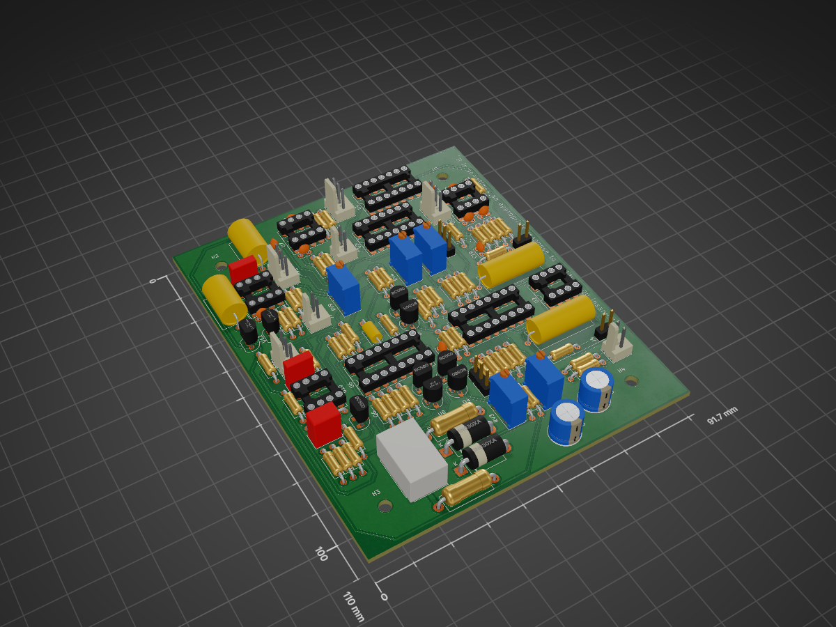
Driven double well is an open-source printed circuit board by aether-machine, from the aether-machine/State-Space-Computer repository on GitHub. It is a 4-layer board of 91.7 × 110 mm with 114 parts on 92 nets, routed with 468 tracks and 0 vias.
It is built around the MPY634KP, TL072 and LM13700M, with the LM334Z, BC560 and BC550 among its other parts. Its parts include 53 resistors, 20 capacitors, 12 ICs, 8 connectors and 6 transistors. It belongs with the audio and music boards of this library.


This repository began it's life as the Oscilloplasm module which existed for a brief time in the Wiard 300 Series format, and has now expanded into a complete and separate take on the audio synthesis paradigm based on continuous computing techniques that occur in the physical and non-physical domains. Here, we present both a general method to solve computing problems using electronic means, and ready made solutions to build and install yourself. The licensing is strictly for non-commercial use only, e.g. education, DIY.
The place to begin is the representation of physical phenomena as periodic information, starting in two dimensions as sound waves and following through into three dimensional particles as persistant standing wave patterns that make up our physical universe. This representation can be done in maths using differential equations, from simple linear ordinary differential equations (ODEs) that describe electron shell configurations, into complex non-linear partial differential equations (PDEs) that can describe motion in a body of water, likely with multiple flow velocities and different viscosities. At the most extreme form, a single equation might be able to describe the entire universe, for example reaction-diffusion equations can give rise to cell like growth.
The primitive in analog computing is the state variable, which appears in both the harmonic oscillator (sine wave) and the multimode filter. Mathematically:
$$ \frac{d^2x}{dt^2} + 2\gamma \frac{dx}{dt} + \omega^2 x = F(t) $$
Where ω = 2πf is the angular frequency of the sine wave and the first derivative x' controls damping or growth. To solve in analog form, the second differential x'' (with respect to time) is passed through two voltage controlled integrators, each comprised of a variable transconductance stage, an opamp and a capacitor as a memory cell, with the inversion of the x output connected to the input to solve. This is the general form of solving ODEs using electronic means, to re-arrange in terms of the lowest order derivative, assume that it exists, and then solve by parts using cascaded integrator stages, the final integrator stage then represents the solution and this is used as the input to complete the cycle.
The harmonic oscillator circuit here is unique to the system, a self stablizing sine wave based around a trig identity for instant in the loop gain correction:
$$ sin^2 + cos^2 - 1 = 0 $$
Using two Gilbert Cell mulitpliers and a zener diode stabilized DC reference, this generates a real time error value which can be used to modulate the oscillator loop gain and maintain long term amplitude stability, as well as two second harmonic outputs for the sine and cosine portions of the waveform. The complete equation with stabilization is:
$$ \frac{d^2 x}{dt^2} + 2k\epsilon \frac{dx}{dt} + \left(\omega^2 + k^2\epsilon^2\right)x = 0 $$
Output oscillator is a variable harmonic wavetable that solves Legendre's Ordinary Differential Equation in real time:
$$ (1 - t^2) \frac{d^2x}{dt^2} - 2t \omega \frac{dx}{dt} + (\omega^2 - l(l+1))x = 0 $$
Where L represents the azimuthal quantum number, thus generating polynomial functions in a completely novel (and sometimes frustrating) way.
The stabilization technique in this oscillator is also state of the art, although there is a compromise between harmonic distortion and ampltiude distortion. Ampltitude distortion as the RMS to DC converter gets stuck in a modulation loop is probably the more destructive force here for audio work. It can be mitigated by avoiding rapid changes in oscillator frequency, perhaps by using a slew limiter on your seqeuncer.
Output oscillator uses four quadrant multipliers and is designed for through zero behaviour.

| Qty | Value | Footprint | References |
|---|---|---|---|
| 20 | 10k | Resistor_THT:R_Axial_DIN0207_L6.3mm_D2.5mm_P10.16mm_Horizontal | R10, R13, R14, R16, R17, R22, R27, R29, R30, R31, R32, R38, R41, R42, R43, R44 +4 |
| 15 | 1k | Resistor_THT:R_Axial_DIN0207_L6.3mm_D2.5mm_P10.16mm_Horizontal | R1, R2, R3, R4, R12, R23, R24, R25, R28, R33, R36, R37, R46, R51, R52 |
| 10 | C | Capacitor_THT:C_Disc_D3.4mm_W2.1mm_P2.50mm | C7, C8, C9, C10, C11, C13, C16, C18, C19, C20 |
| 6 | 100 | Resistor_THT:R_Axial_DIN0207_L6.3mm_D2.5mm_P10.16mm_Horizontal | R21, R34, R35, R47, R48, R50 |
| 5 | BC560 | Package_TO_SOT_THT:TO-92_HandSolder | Q1, Q2, Q3, Q4, Q5 |
| 5 | R_Potentiometer | Potentiometer_THT:Potentiometer_Bourns_3296Y_Vertical | RV2, RV3, RV4, RV5, RV9 |
| 5 | TL072 | Package_DIP:DIP-8_W7.62mm_Socket_LongPads | U2, U5, U7, U10, U11 |
| 4 | MountingHole | MountingHole:MountingHole_3.2mm_M3 | H1, H2, H3, H4 |
| 4 | R_Potentiometer | Connector_Molex:Molex_KK-254_AE-6410-03A_1x03_P2.54mm_Vertical | RV1, RV6, RV7, RV8 |
| 3 | Conn_01x02 | Connector_Molex:Molex_KK-254_AE-6410-02A_1x02_P2.54mm_Vertical | J3, J7, J8 |
| 2 | 1N630xA | Diode_THT:D_DO-201AE_P12.70mm_Horizontal | D1, D2 |
| 2 | 200k | Resistor_THT:R_Axial_DIN0207_L6.3mm_D2.5mm_P10.16mm_Horizontal | R15, R18 |
| 2 | C | Capacitor_THT:C_Rect_L7.2mm_W2.5mm_P5.00mm_FKS2_FKP2_MKS2_MKP2 | C6, C12 |
| 2 | C | Capacitor_THT:C_Axial_L12.0mm_D7.5mm_P15.00mm_Horizontal | C14, C15 |
| 2 | C | Capacitor_THT:C_Axial_L17.0mm_D7.0mm_P20.00mm_Horizontal | C1, C2 |
| 2 | C_Polarized | Capacitor_THT:CP_Radial_D8.0mm_P5.00mm | C3, C5 |
| 2 | Conn_01x02 | Connector_PinHeader_2.54mm:PinHeader_1x02_P2.54mm_Vertical | J4, J5 |
| 2 | Conn_01x03 | Connector_PinHeader_2.54mm:PinHeader_1x03_P2.54mm_Vertical | J2, J6 |
| 2 | LM13700 | Package_DIP:DIP-16_W7.62mm_Socket_LongPads | U1, U6 |
| 2 | LM4040LP-10 | Package_TO_SOT_THT:TO-92_Inline | U12, U13 |
| 2 | MPY634KP | Package_DIP:DIP-14_W7.62mm_Socket_LongPads | U3, U4 |
| 2 | R | Resistor_THT:R_Axial_DIN0207_L6.3mm_D2.5mm_P10.16mm_Horizontal | R5, R11 |
| 2 | R | Resistor_THT:R_Axial_DIN0414_L11.9mm_D4.5mm_P15.24mm_Horizontal | R19, R20 |
| 2 | ~ | Resistor_THT:R_Axial_DIN0207_L6.3mm_D2.5mm_P10.16mm_Horizontal | R39, R40 |
| 1 | 1meg | Resistor_THT:R_Axial_DIN0207_L6.3mm_D2.5mm_P10.16mm_Horizontal | R53 |
| 1 | 2.5k | Resistor_THT:R_Axial_DIN0207_L6.3mm_D2.5mm_P10.16mm_Horizontal | R7 |
| 1 | 4.7k | Resistor_THT:R_Axial_DIN0207_L6.3mm_D2.5mm_P10.16mm_Horizontal | R49 |
| 1 | 5k | Resistor_THT:R_Axial_DIN0207_L6.3mm_D2.5mm_P10.16mm_Horizontal | R26 |
| 1 | BC550 | Package_TO_SOT_THT:TO-92_HandSolder | Q6 |
| 1 | C | Capacitor_THT:C_Rect_L7.2mm_W4.5mm_P5.00mm_FKS2_FKP2_MKS2_MKP2 | C17 |
| 1 | C | Capacitor_THT:C_Axial_L5.1mm_D3.1mm_P10.00mm_Horizontal | C4 |
| 1 | Conn_01x04 | Connector_Molex:Molex_KK-396_A-41791-0004_1x04_P3.96mm_Vertical | J1 |
| 1 | LM334Z | Package_TO_SOT_THT:TO-92_HandSolder | U8 |
It measures 91.7 × 110 mm and has 4 copper layers, 1.61 mm thick.
114 parts, built around the MPY634KP, TL072, LM13700M and LM334Z. The full list of its parts is on this page, with links to each part's symbol and footprint where PCBKit's library has them.
From the aether-machine/State-Space-Computer repository on GitHub, at the commit this page was made from: the board is boards/driven-double-well/driven-double-well.kicad_pcb and its schematic boards/driven-double-well/driven-double-well.kicad_sch. PCBKit opens the board in the browser, with nothing to install.
Its repository states no licence, so its author keeps all rights: ask aether-machine before reusing the design.


JordanAceto/modulation_source
Eurorack compatible pcb with sine/square VCLFO, white and pink noise, and sample & hold


bubbajfett/kicad-guitar-pedals
collection of guitar pedal PCB layouts in kicad

mesotokyo/nubuf3
MST DRIVE (Nutube Powered Booster/Overdrive) schematic and PCB for KiCAD

ManikantanRS03/Mani_IITPKD_Research
Stochastic Resonance in Ferroelectric