
2 layers168.9 × 123.3 mm
OEM ECU
aeonSolutions/AeonLabs-AI-Volvo-MKII-Open-Hardware
Volvo MKII Open Hardware
296 parts161CC0-1.0

python import pandas as pd from importlib import reload import matplotlib.pyplot as plt import numpy as np from IPython.display import display
Ct4 is an open-source printed circuit board by mckennatim, from the mckennatim/ct4 repository on GitHub. It is a 4-layer board of 76.2 × 104.1 mm with 34 parts on 48 nets, routed with 144 tracks and 0 vias.
It is built around the ADS1115. Its parts include 12 resistors, 8 capacitors, 6 ICs and 4 connectors.
import pandas as pd
from importlib import reload
import matplotlib.pyplot as plt
import numpy as np
from IPython.display import displayDesign a 4 CT energy monitor for 4 circuits. On hand are a number of 15A/1v and 20A/1v current transformers. When the CT has that kind of designation, the burden resistor is already included. (If not calculate burden resistor below in ref)
Best Resources for Explanation:
Electronics Textbooks:
Online Resources:
YouTube Channels:
*lots of holes too big
Consider the current range of the heatpump we want to monitor.
# unit label data
total_A = 10.9
compressor_A = 9.2
fan_A = .3
ampacity = 13.2
indoor_Fan_A = .35
indoor_model = "ASUH09KTAS"
indoor_serial = "LDA000334"
outdoor_model = "AOUH09KTAP1"
outdoor_serial = "LDN000103"
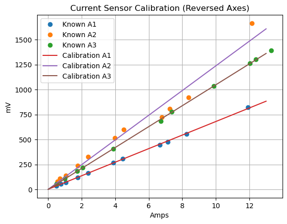
Test (120V) hair drier, fan, immersion blender and jig saw to find mV produced by sensor, for each current produced as measured by clamp on current meter.
# fan: fh,fl immersion blender: im, hairdrier lo hi, cool, warm, hi: dlc, dlw, dlh, dlh, dhh
sources = ["fh","fl+im", "dlc", "dhc", "dhc+fh+im", "dlw", "dlw+fh+im", "dlh", "dlh+fh+im" "dhh"]
known_A1 = [.48, .75, 1.04, 1.75, 2.39, 3.90, 4.45, 6.65, 7.12, 8.25, 11.93]
known_A2 = [.54, .71, 1.04, 1.75, 2.39, 3.99, 4.52, 6.77, 7.25, 8.36, 12.15]
known_A3 = [.48, 1.0, 1.72, 2.06, 3.88, 6.72, 7.38, 9.88, 12.02, 12.4, 13.31]
mv_A1 = [36, 54,72, 121, 165, 268, 306, 448, 478, 554, 821]
mv_A2 = [78, 110, 141, 238, 328, 517, 600, 723, 810, 920, 1665]
mv_A3 = [53, 108, 183, 219, 406, 684, 778, 1037, 1264, 1305, 1391]
df1 = pd.DataFrame({"A": known_A1, "mv": mv_A1})
df2 = pd.DataFrame({"A": known_A2, "mv": mv_A2})
df3 = pd.DataFrame({"A": known_A3, "mv": mv_A3})
coeffs1 = np.polyfit(df1["A"], df1["mv"], 1)
coeffs2 = np.polyfit(df2["A"], df2["mv"], 1)
coeffs3 = np.polyfit(df3["A"], df3["mv"], 1)
poly1 = np.poly1d(coeffs1)
poly2 = np.poly1d(coeffs2)
poly3 = np.poly1d(coeffs3)
print("Calibration Polynomial 1 (A1): ")
print(poly1)
print("Calibration Polynomial 2 (A2): ")
print(poly2)
print("Calibration Polynomial 3 (A3): ")
print(poly3)
print(poly2) Cell In[11], line 50
plt.plot(df2["A"], df2["mv"], "o", label="Known A2")
^
IndentationError: unexpected indentsources = ["fh","fl+im", "dlc", "dhc", "dhc+fh+im", "dlw", "dlw+fh+im", "dlh", "dlh+fh+im", "dhh"]
known_A1 = [.48, .75, 1.04, 1.75, 2.39, 3.90, 4.45, 6.65, 7.12, 8.25, 11.93]
known_A2 = [.54, .71, 1.04, 1.75, 2.39, 3.99, 4.52, 6.77, 7.25, 8.36, 12.15]
known_A3 = [.48, 1.0, 1.72, 2.06, 3.88, 6.72, 7.38, 9.88, 12.02, 12.4, 13.31]
mv_A1 = [36, 54,72, 121, 165, 268, 306, 448, 478, 554, 821]
mv_A2 = [78, 110, 141, 238, 328, 517, 600, 723, 810, 920, 1665]
mv_A3 = [53, 108, 183, 219, 406, 684, 778, 1037, 1264, 1305, 1391]
df1 = pd.DataFrame({"A": known_A1, "mv": mv_A1})
df2 = pd.DataFrame({"A": known_A2, "mv": mv_A2})
df3 = pd.DataFrame({"A": known_A3, "mv": mv_A3})
coeffs1 = np.polyfit(df1["A"], df1["mv"], 1)
coeffs2 = np.polyfit(df2["A"], df2["mv"], 1)
coeffs3 = np.polyfit(df3["A"], df3["mv"], 1)
poly1 = np.poly1d(coeffs1)
poly2 = np.poly1d(coeffs2)
poly3 = np.poly1d(coeffs3)
print("Calibration Polynomial 1 (A1): ")
print(poly1)
print("Calibration Polynomial 2 (A2): ")
print(poly2)
print("Calibration Polynomial 3 (A3): ")
print(poly3)
def A_to_mv1(A):
return poly1(A)Calibration Polynomial 1 (A1):
67.85 x + 1.626
Calibration Polynomial 2 (A2):
123.6 x + 1.254
Calibration Polynomial 3 (A3):
104.7 x + 0.9221
[67.85287623 1.62603625]# y = mx + b
m = 104.7
b = .9221
x = 10.9
y = 800
c = (y-b)/m
print(f"Calculated current for {y:0.2f} mV: {c:0.2f} A")Calculated current for 800.00 mV: 7.63 AThe 1uF capacitor on S blocks the DC component of the bias voltage from dragging down and shorting out through the 53ohm internal R of the CT (as measured at the pins)
The load impedance isn't just the 53Ω CT - it's the parallel combination of:
Since 60kΩ >> 53Ω, the AC impedance is essentially 53Ω.
But actually, for the cutoff frequency, what matters is the impedance that C1 sees:
C1 sees: CT (53Ω) in series with [R1 || R2] = 53Ω + 53kΩ ≈ 53kΩ
for the high-pass filter cutoff, the relevant impedance is the bias network (R1||R2 = 53kΩ)
(The 53Ω only matters for loading the voltage divider with AC current, which is minimal with 60kΩ bias resistors. )
Rule of Thumb: Choose fc to be 1/10th of your lowest frequency of interest for minimal signal loss.
For fc = 6 Hz: C = 1 / (2π × 53,000 × 6) ≈ 0.5 µF
Round up to 1uF


#### calculating values


```python
R1 = 82000
R2 = 153000
Rct =53

R1llR2 = (R1*R2)/(R1+R2)
print(f"Parallel resistance of R1 and R2: {R1llR2:0.1f} ohms")
Vbias = 2.5 * R2 /(R1+R2)
print(f"Bias voltage at divider point: {Vbias:0.3f} V")

Rctll_R1llR2 = (Rct*R1llR2)/(Rct+R1llR2)
print(f"Total resistance seen at bias point with load: {Rctll_R1llR2:0.1f} ohms")

fc = 6  # hz 1/10 of 60hz
C1 = 1 / (2*3.14159 * R1llR2 * fc)

print(f"Capacitance needed: {C1*1e6:0.2f} uF")Parallel resistance of R1 and R2: 53387.2 ohms
Bias voltage at divider point: 1.628 V
Total resistance seen at bias point with load: 52.9 ohms
Capacitance needed: 0.50 uFTo account for the load, you need to ensure the resistor provides enough current for both the LM4040’s minimum operating current and the current drawn by your voltage divider (and any other load).
Choose the next lower standard value to ensure enough current (e.g., 10 kΩ).
Iload = 2.5/(100000+150000)
print(f"Load current through resistor: {Iload*1000} mA")
Imin = 60e-6
print(f"Minimum current through resistor with load: {Imin*1000:0.3f} mA")
Itotal = Imin + Iload
print(f"Total current through resistor with load: {Itotal*1000:0.3f} mA")
R=(3.3-2.5)/Itotal
print(f"Resistor value to set minimum current with load: {R:0.1f} ohms")Load current through resistor: 0.01 mA
Minimum current through resistor with load: 0.060 mA
Total current through resistor with load: 0.070 mA
Resistor value to set minimum current with load: 11428.6 ohmsChanged the default terminal in vscode to cmd. cmd-shift-p Terminal:Select default profile
cmd couldn't find where python
Platformio uses its own penv python. It complained about missing a library. Since cmd uses conda, pip would have used the active conda env pip and put it in the wrong place. To use Platformio's python:
from cmd run platformio system info to see where python is and it is
A fatal error occurred: Failed to connect to ESP32: Wrong boot mode detected (0x13)! The chip needs to be in download mode
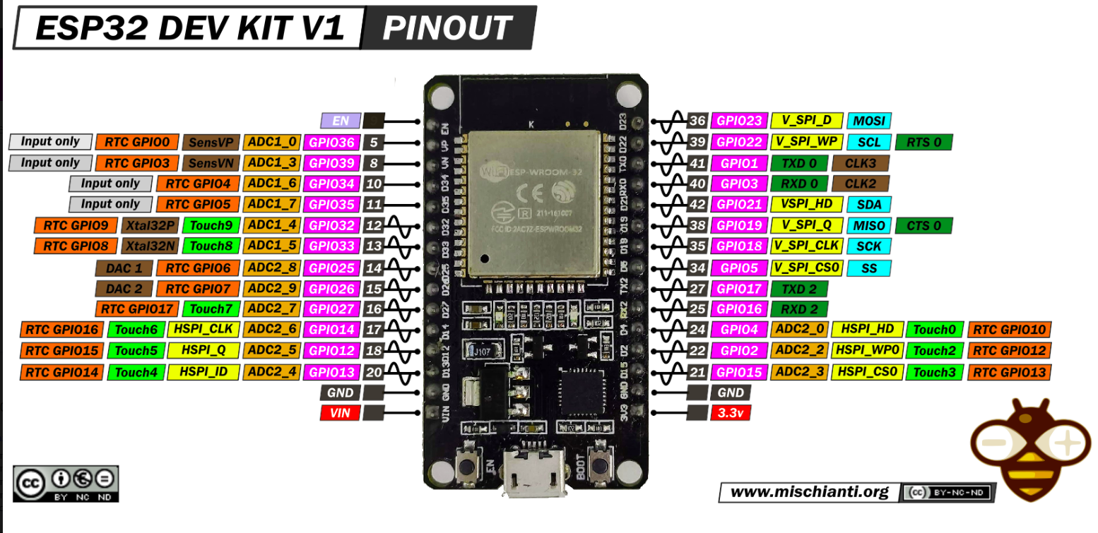
CONFIGURATION: https://docs.platformio.org/page/boards/espressif32/esp32doit-devkit-v1.html
PLATFORM: Espressif 32 (6.12.0) > DOIT ESP32 DEVKIT V1
HARDWARE: ESP32 240MHz, 320KB RAM, 4MB Flash
declare functions defined later before setup
Take 500 samples: zeroOffsetADC is the average of the digital counts of the ADC at 0V
zeroOffsetADC = sum / numSamples;
For the ADS1115, each count at GAIN_ONE (±4.096 V) is 0.125 mV
Calibrating zero offset... ensure CT is not measuring any current
Zero offset calibrated: 12895.45 ADC counts
This corresponds to: 1.612 V bias
counts0 = 12895.45
volts0 = counts0 * 0.000125
print(f"Zero offset: {counts0:0.2f} counts = {volts0:0.3f} V")Zero offset: 12895.45 counts = 1.612 Vcounts7_1A = 10704
volts7_1A = .734
x = volts7_1A / counts7_1A
print(f"x = {x:0.8f},{x*2:0.8f}")x = 0.00006857,0.00013714cz= 16
vz=.0000015
x = vz/cz
print(f"x = {x:0.8f},{x*2:0.8f}") x = 0.00000009,0.00000019goto ct4.ipynb for specific info
| Qty | Value | Footprint | References |
|---|---|---|---|
| 4 | .1uF | Capacitor_THT:C_Disc_D7.5mm_W5.0mm_P5.00mm | C2, C3, C5, C7 |
| 4 | 10K | Resistor_THT:R_Axial_DIN0204_L3.6mm_D1.6mm_P7.62mm_Horizontal | R3, R4, R7, R10 |
| 4 | 153K | Resistor_THT:R_Axial_DIN0204_L3.6mm_D1.6mm_P7.62mm_Horizontal | R1, R6, R9, R12 |
| 4 | 1uF | Capacitor_THT:C_Disc_D7.5mm_W5.0mm_P5.00mm | C1, C4, C6, C8 |
| 4 | 2.5 | Package_TO_SOT_THT:TO-92_Inline | U1, U3, U5, U6 |
| 4 | 82K | Resistor_THT:R_Axial_DIN0204_L3.6mm_D1.6mm_P7.62mm_Horizontal | R2, R5, R8, R11 |
| 4 | AudioJack3 | footprints:audiojack_female_3pin_3.5mm | J1, J2, J3, J4 |
| 4 | MountingHole | MountingHole:MountingHole_3.5mm | H1, H2, H3, H4 |
| 1 | ADS1115 | footprints:ADC1115_ADC_Module | U2 |
| 1 | ~ | footprints:ESP32_30pin | U4 |
It measures 76.2 × 104.1 mm and has 4 copper layers, 1.6 mm thick.
34 parts, built around the ADS1115. The full list of its parts is on this page, with links to each part's symbol and footprint where PCBKit's library has them.
From the mckennatim/ct4 repository on GitHub, at the commit this page was made from: the board is kicad8/ct4/ct4.kicad_pcb and its schematic kicad8/ct4/breadboard/breadboard.kicad_sch. PCBKit opens the board in the browser, with nothing to install.
Its repository states no licence, so its author keeps all rights: ask mckennatim before reusing the design.
aeonSolutions/AeonLabs-AI-Volvo-MKII-Open-Hardware
Volvo MKII Open Hardware


rin67630/Drok-Juntek-on-steroids
Extend the possibilities of cheap digital power supplies with a WiFi module

sdylewski/Analog-Redial
A circuit board for old telephones to come back to life. Plug one or two phones in, and you can call the other phone, use bluetooth, connect to others via voip, and do a variety of other things with a plain old rotary…


ToneAlchemy/BiasPro
A professional-grade, dual-probe Arduino Bias Meter for guitar tube amplifiers. Open source hardware & firmware

mikelawrence/esphome-indoor-multi-sensor-hardware
ESPHome Indoor Multi-Sensor hardware. This design supports Radar/PIR Presence, Temperature, Humidity, Pressure, Light, CO2, CO, VOC, NOX and PM sensors.
