2 layers52.3 × 10.5 mm
StackLink
gusmanb/logicanalyzer
24 channel, 100Msps logic analyzer hardware and software
29 parts5.1kGPL-3.0

 ardagurbuuz/Lead-Compensator2
Analog lead compensator for a second-order plant to improve transient performance (reduced overshoot, faster settling).
Lead Compensator is an open-source printed circuit board by ardagurbuuz, from the ardagurbuuz/Lead-Compensator repository on GitHub. It is a 2-layer board of 88.5 × 57.5 mm with 29 parts on 22 nets, routed with 122 tracks and 4 vias.
Its parts include 15 resistors, 4 capacitors, 2 ICs and 1 switch. It belongs with the audio and music boards of this library.
This repository documents an end-to-end control + hardware workflow: designing a lead compensator, validating it at model-level (MATLAB/Simulink) and circuit-level (SPICE tools), and implementing it as an op-amp analog controller on a KiCad PCB.
A benchmark plant model is used as the baseline system:
$$ G(s)=\frac{2}{s(s+1)} $$
The project compares two closed-loop configurations under the same input:
This block-level structure is implemented and cross-validated across tools:
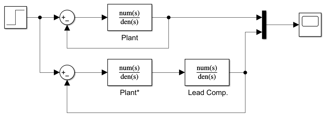
A lead compensator adds phase lead in a chosen frequency range. Practically, it helps achieve:
The plant
G(s) = 2 / (s(s+1))
was chosen deliberately because it is a clean benchmark that exposes the core trade-offs a lead compensator is meant to address:
1/s term introduces an integrator, which is a common structure when the system output represents an accumulated quantity (position/angle/level).1/(s+1) term adds a dominant first-order lag, a very typical dynamic limitation in real systems.In short: it’s an intentional baseline that makes controller impact measurable and transferable.
The project is built around a single, clear comparison:
with the intent to improve transient performance (reduced overshoot, faster settling) while keeping the design implementable in analog hardware.
The compensator was selected using Root Locus–based design, specifically:
This approach links performance objectives directly to pole locations and results in a compensator that is both analyzable and implementable.
This project intentionally uses multiple tools because each one answers a different question. Using only one would leave blind spots.
MATLAB is used to verify the math: pole/zero placement logic, gain consistency, and quick numeric checks. This prevents “it looks right” errors before simulation.
Simulink is used to observe signals and step responses in a clean block-diagram environment and to compare compensated vs. uncompensated outputs under the same stimulus.
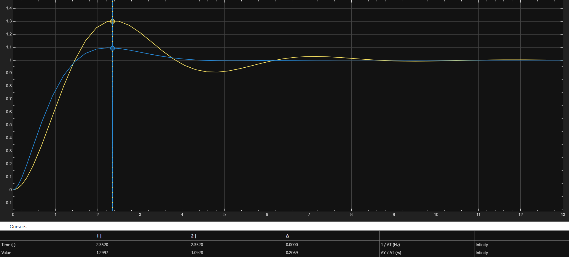
LTspice is used to rebuild the control structure as ideal analog circuits, for two reasons:
Proteus is used as the “last realism check” before committing to PCB:
In short:
After validating behavior in simulation, the controller is implemented using op-amp analog circuitry and captured in KiCad as:
A key constraint throughout the hardware step is real-world component availability:
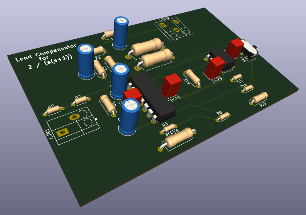
Fabrication note: The current PCB is a 2-layer design. If single-sided fabrication is required, it will generally need rerouting and/or jumpers.
This repo is structured so each stage can be opened independently.
Folder: matlab-simulink/
lead_compensator.m → calculation/verification scriptplant_comp.slx → compensated system modeluncomp_step_response.slx → baseline (plant-only) response modelOpen in MATLAB/Simulink and run the script/models to reproduce the response comparison.
Folder: ltspice/
lead-compensator.asc → circuit fileOpen in LTspice and run the transient simulation to inspect waveforms.
Folder: proteus/
lead-compensator.pdsprj → project file (includes switch-based comparison setup)Open in Proteus, run simulation, and toggle the switch to compare modes.
Folder: kicad/
lead-compensator.kicad_sch → schematiclead-compensator.kicad_pcb → PCB layoutlead-compensator.kicad_pro → project settingsOpen the .kicad_pro project file in KiCad, then inspect schematic/PCB.
docs/images/ → curated images used in READMEkicad/ → KiCad schematic + PCBmatlab-simulink/ → MATLAB + Simulink modelsltspice/ → LTspice circuit (SPICE tool)proteus/ → Proteus project (SPICE tool)MATLAB, Simulink, LTspice (SPICE tool), Proteus (SPICE tool), KiCad
Root Locus, dominant poles, angle condition, magnitude condition, lead compensator, transient response, overshoot, settling time, circuit-level validation, op-amp analog implementation, PCB design, DRC-clean layout, end-to-end engineering workflow.
| Qty | Value | Footprint | References |
|---|---|---|---|
| 5 | 100k | Resistor_THT:R_Axial_DIN0207_L6.3mm_D2.5mm_P7.62mm_Horizontal | R1, R2, R3, R4, R13 |
| 4 | 100n | Capacitor_THT:C_Rect_L4.6mm_W3.8mm_P2.50mm_MKS02_FKP02 | CDCP5, CDCP6, CDCP7, CDCP8 |
| 4 | 10k | Resistor_THT:R_Axial_DIN0204_L3.6mm_D1.6mm_P5.08mm_Horizontal | R5, R6, R7, R8 |
| 2 | 10u | Capacitor_THT:C_Radial_D5.0mm_H11.0mm_P2.00mm | C1, C2 |
| 2 | 1k | Resistor_THT:R_Axial_DIN0204_L3.6mm_D1.6mm_P5.08mm_Horizontal | R14, R15 |
| 2 | 1u | Capacitor_THT:C_Radial_D5.0mm_H11.0mm_P2.00mm | C3, C4 |
| 2 | 330k | Resistor_THT:R_Axial_DIN0414_L11.9mm_D4.5mm_P15.24mm_Horizontal | R10, R11 |
| 1 | 10M | Resistor_THT:R_Axial_DIN0309_L9.0mm_D3.2mm_P12.70mm_Horizontal | RLK16 |
| 1 | 33k | Resistor_THT:R_Axial_DIN0207_L6.3mm_D2.5mm_P7.62mm_Horizontal | R12 |
| 1 | 560k | Resistor_THT:R_Axial_DIN0207_L6.3mm_D2.5mm_P7.62mm_Horizontal | R9 |
| 1 | Conn_01x02 | TerminalBlock_Degson:TerminalBlock_Degson_DG250-3.5-02P_1x02_P3.50mm_45Degree | J_IN1 |
| 1 | Conn_01x03 | TerminalBlock_Degson:TerminalBlock_Degson_DG250-3.5-03P_1x03_P3.50mm_45Degree | J_PWR2 |
| 1 | SW_Slide_DPDT | Button_Switch_THT:SW_CK_JS202011AQN_DPDT_Angled | SW1 |
| 1 | TL071 | Package_DIP:DIP-8_W7.62mm | U2 |
| 1 | TL074 | Package_DIP:DIP-14_W7.62mm | U1 |
gusmanb/logicanalyzer
24 channel, 100Msps logic analyzer hardware and software

VoronDesign/Voron-Hardware
Cool Hardware designed by the Voron Design group

hoglet67/RGBtoHDMI
Bare-metal Raspberry Pi project that provides pixel-perfect sampling of Retro Computer RGB/YUV video and conversion to HDMI

hackclub/OnBoard
💡 Join 1,000 teenagers and make your first PCB with a $100 grant!

OLIMEX/DIY-LAPTOP
Do It Yourself Open Source Hardware and Software Modular Hacker's Friendly Laptop

UtilitechAS/amsreader-firmware
ESP8266 and ESP32 compatible firmware to read, interpret and publish data to MQTT from smart electrical meters, both DLMS and DSMR is supported


It measures 88.5 × 57.5 mm and has 2 copper layers, 1.6 mm thick.
29 parts. The full list of its parts is on this page, with links to each part's symbol and footprint where PCBKit's library has them.
From the ardagurbuuz/Lead-Compensator repository on GitHub, at the commit this page was made from: the board is kicad/lead-compensator.kicad_pcb and its schematic kicad/lead-compensator.kicad_sch. PCBKit opens the board in the browser, with nothing to install.
Its repository states no licence, so its author keeps all rights: ask ardagurbuuz before reusing the design.