This signal of the heartbeat, in the form of the "PQRST" complex as seen with Figure 1, is what needs to be detected in order to find important information about a patient's heart.
ECG Project Josh is an open-source printed circuit board by TallesSantosCUBoulder, from the TallesSantosCUBoulder/ECEN4532_DSPLab_Spring2026_ECG_Project repository on GitHub, published under the MIT licence. It is a 2-layer board of 66.5 × 53 mm with 35 parts on 27 nets, routed with 152 tracks and 0 vias.
It is built around the AD623AN. Its parts include 19 resistors, 10 capacitors, 3 ICs and 3 connectors.
ECEN4532: Digital Signal Processing Laboratory (Spring 2026) Instructor: Talles Santos Students: Alyssa Jackson
Joshua Thomas
Emilie Teel
Introduction
An electrocardiogram (often shortened to ECG or EKG) procedure is a quick and simple test that is designed to record the eletrical signal from a patient's beating heart and use it to find its natural rhythmic cycle [1]. By placing electrodes aroud the patient's chest, arms, and/or legs, a circuit is created with the heart as the voltage source the contractions caused by electricity are pickeed up by the electrodes and sent to a circuit.
Figure 1: A diagram of the different parts of a heartbeat that are searched for during an ECG test [2].
This signal of the heartbeat, in the form of the "PQRST" complex as seen with Figure 1, is what needs to be detected in order to find important information about a patient's heart. Things like poor blood flow, arrhythmias, heart attacks, and thickened heart walls, can be picked up, seen, and diagnosed accurately with this type of circuit [4].
The goal of this project is not only to build an analog circuit that can pick up the signals of a heartbeat, but to then transmit that data using an Arduino Uno to MATLAB that will then visual said data from the heart and calculate the BPM (or the beats per minute) from the received signal.
Methodology
Hardware
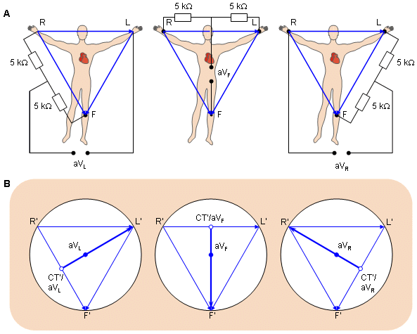
Figure 2: A diagram of the circuit that a body completes based on the position of the electrodes. A) represents the circuit on a body while B) shows the connections in the image space. [3]
As can be seen in Figure 2, the basic premise of the ECG Circuit itself involves building a voltage divider with the heart in order to pick up the signals ans input it into the circuit.
Circuit Schematic
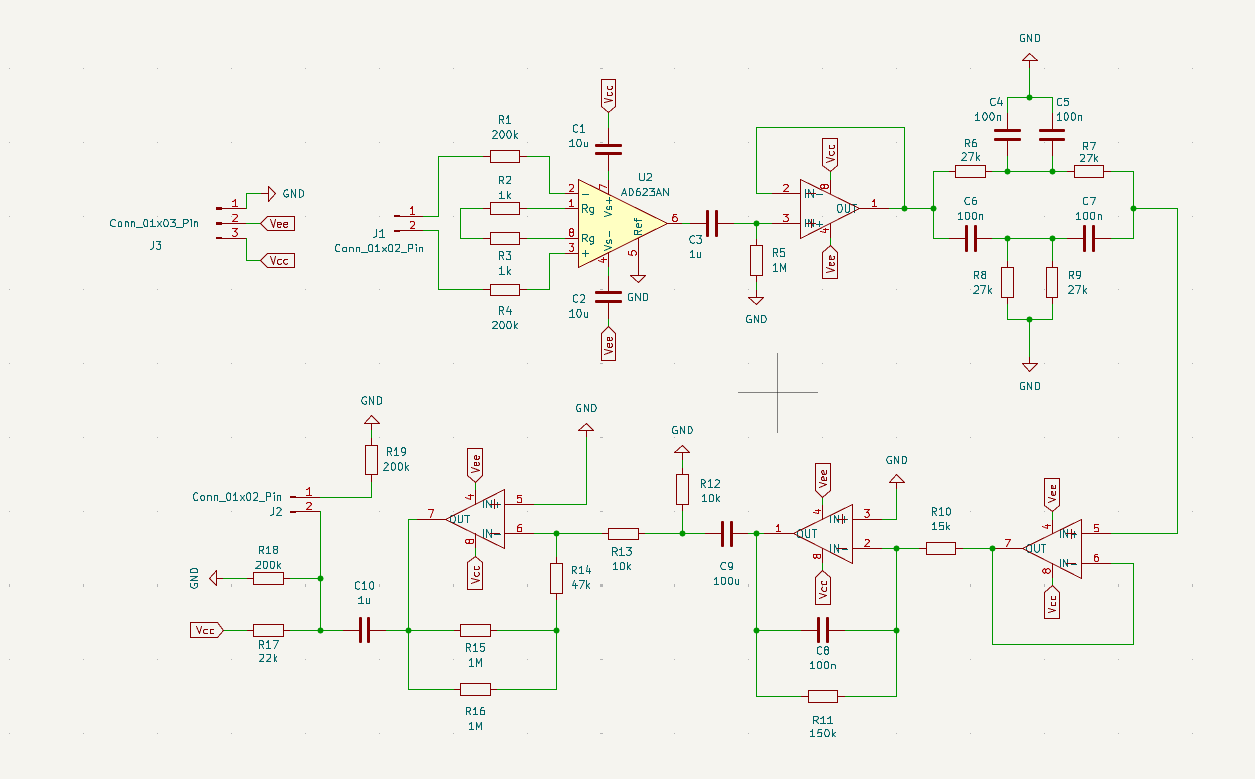
To gather the heart rate information from the body leads are attatched to the patient and then connected to an analog circuit to filter and amplify the data coming in from the leads. This circuit is used as a form of preprocessing to alow for a more precise reading from the microcontroller. Below is the schematic of the ECG circuit that was used in its design.
The Schematic of the circuit is broken into parts each playing a role in the amplification, filtering, or offset of the signal for later interpretation. The first segment of the schematic is an instrumentation amplifier to take the very weak signal from the body and give it gain to allow for filtering. The second step is a passive high pass filter made of a capacitor and resistor. This stage is used to reduce interferance from body roll and breathing, and to remove dc offset from the signal. The next stage is a buffer to isolate previos stages from feedback. The following stage is a 60hz notch filter. This filter has a high attenuation of the 60 hz signal to remove interferance from main powr in the room as it is the biggest source of interferance in the signal. This is then fed into a buffer to once again isolate the filter from future stages. The subsiquent stage is an active low pass filter to further attenuate high frequencies such as 60hz and to remove any noise from frequencies not produced by heartrate. The final stage is an inverting amplifier to further amplify the signal for processing, and it is combined with a circuit to add offset so the microcontroller can read the signal.
PCB Design
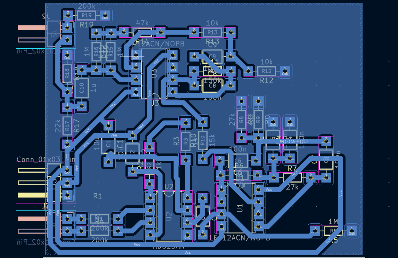
To buid the circuit in hardware the schematic was then used to design the PCB to physically implement the circuit. Below is the PCB schematic that was used in this project.
There was an itterative process used in designing the layout for the PCB. The software used for this was KICAD, and in this software it has the ability to select pieces from the schematic to then place on the PCB. So the circuit was designed piece by piece for each module. The circuit looped arround starting at the bottom left corner with the inputs and moving on to the top left for the output. each of the op amps used were dual op amps and therefor the sequential modules were able to make use of the two amplifiers vutting down on the size of the circuit. The difficult part of the design was making sure that all power inputs and ground planes were connected propperly. Through trial and error the above circuit was compiled.
The hardware was not able to be completed at the time of this paper, but the components have been selected and they will be soldered to the pcb to complete the analog circuit.
Testing the Hardware
At the time of this paper the circuit was not able to be made due to some issues with the milling machine, but there are further steps for future use when the machine is up and running. The future plans for testing is to print out the PCB, solder on the components, and connect the completed circuit to the simulator and then to one of us to test the output. The output of the circuit will be observed from the ocilloscope and a passed test will be a test that shows a similar result to the already working breadboard circuit. The report will be updated with this information when the tests have been run.
Software
For the software side of things, an Arduino Uno R3 was used to take that normalized heartbeat signal, or a simple test signal generated from a function generator, that ranges from 0 to 5V and transmit the data to MATLAB via packets. The packets act like individual bundles of data that are all sent to the host computer running MATLAB in order instead of in a constant real time stream that would take more processing power and lead to potential data errors.
But before the data is sent over, the MATLAB script must be formatted to in order to gather the data coming in from the Arduino at the correct speed and sampling frequency:
matlab
% define port; check whatever port the Arduino is connected to
% and uncomment that one while commenting the other ports
portName = serialportlist("available");
% portName = '/dev/ttyACM0' ;
% portName = '/dev/ttyACM1' ;
portName = '/dev/ttyUSB0' ;

% open port
fp = serialport(portName,115200);

% settings
fs = 1 / (3e-3) ;                          % sampling frequency of the arduino
sizeBufferArduino = 20 ;                   % from arduino code
t_Buffer = 10.0 ;                          % in seconds
nSamplesBuffer = round(t_Buffer*fs) ;      % nSamples of the circular buffer in the matlab script
bits2volts = 5/(2^10-1) ;                  % convertion from bits to volts (arduino uno 10 bits)

% initialing variables
CircularBuffer = zeros(nSamplesBuffer,1);
vecSamples = 0 ;
count=1;
Code Snipet 1: The first lines from the MATLAB script 'read_serial_Nsamples_buffer.m'. These lines work to format everything from the baud rate being received, the sampling frequency that the signal is being measured at, the size of the data packets that are recieved at once, conversion of the Arduino value from 0 to 5 volts, and other variables needed in the plotting of the data in real-time.
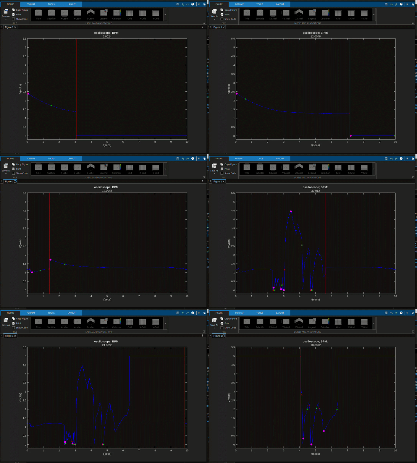
That packet of 20 individual values from the Arduino is sent to a loop that can't be left without a Serial port disconnection or a manual code end caused by the user. That loop constantly looks for the start of the new incoming packet, packet into a vector that MATLAB can tranversed, enters that vector being evaluated, turns the value into a voltage thanks to the data conversion with a time attached to the value, and finally plotted on a constantly updating graph of voltage vs. time. A circular buffer is used so that a constant stream of voltages can be plotted in an ever-rotating plot that can be seen in Figure 3 below.
Figure 3: A gif that shows how the plotting of data works on MATLAB. The red vertical line acts as the real-time sweep as the signal gets plotted.
As can also be seen from Figure 3, there are also magneta dots and red and green stars on the signal as well. These are the marks that are meant to point to the what the R peak of a signal is as well as the right(green) and left(red) of that R peak, as explained below:
matlab
% For the best and most accurate data, the inputted signal need to be
% filtered first
function [R_loc, left, right, bpm]=identifyQRSComplex(signal,Fs)


R_loc = [];
left = [];
right = [];
bpm = NaN;
%% Preprocessing the signal for QRS detection
x = signal;

% Removing the DC Offset from the Signal
x = x - mean(x);

% Finding the Time Scale of the Signal
T = 1/Fs;
N = length(x);

t = (0:N-1)*T;

% Normalizing the Signal
Norm_signal = x.^2;
Norm_signal = Norm_signal / max(abs(Norm_signal));
Code Snipet 2: The 'identifyQRSComplex' function used in the MATLAB code to find the bpm, the R location from the QRS complex, and the left and right of the the R location.
The code from the above snipet is the entireity of the function, and it also has the added benefit of being able to calculate the bpm (or the frequency of a signal in the span of a minute) of the input signal, which is displayed at the top of the gif in Figure 3. When combined, the function from Code Snipet 2 and the MATLAB script, the entirity of the code can detect the peaks of a signal, mark its highest point, the immediate left and right of that peak, and the BPM (or the frequency per minute for non-heartbeat signals) of the signal that is detected through the Arduino Uno.
Testing the Software
Testing the programming for both the Arduino and MATLAB itself is pretty simple: connect the Arduino to PC running the MATLAB script and view the real-time output from the A0 pin.
Figure 4: A gif that shows how the plotting of signals to MATLAB. The gif shows the signals from the A0 pin connected to the GND pin, the 5V pin, and just open to the air.
As shown with Figure 4, the signal from the Arduino in the different inputs to the A0 pin. In this test, the BPM from the signal means nothing since the Arduino updating from the inputs was slow due to the packets method, so a different test would be needed to see how the BPM calculation would work.
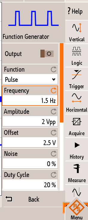
Figure 5: The settings used for the test signal input in the Arduino.
Instead of just having a DC signal and moving it from 5V to GND very fast by hand, a function generator was used instead and set with the parameter as seen in Figure 5. The gif from Figure 3 is the real-time plotting of the signal generated using the information from Figure 5.
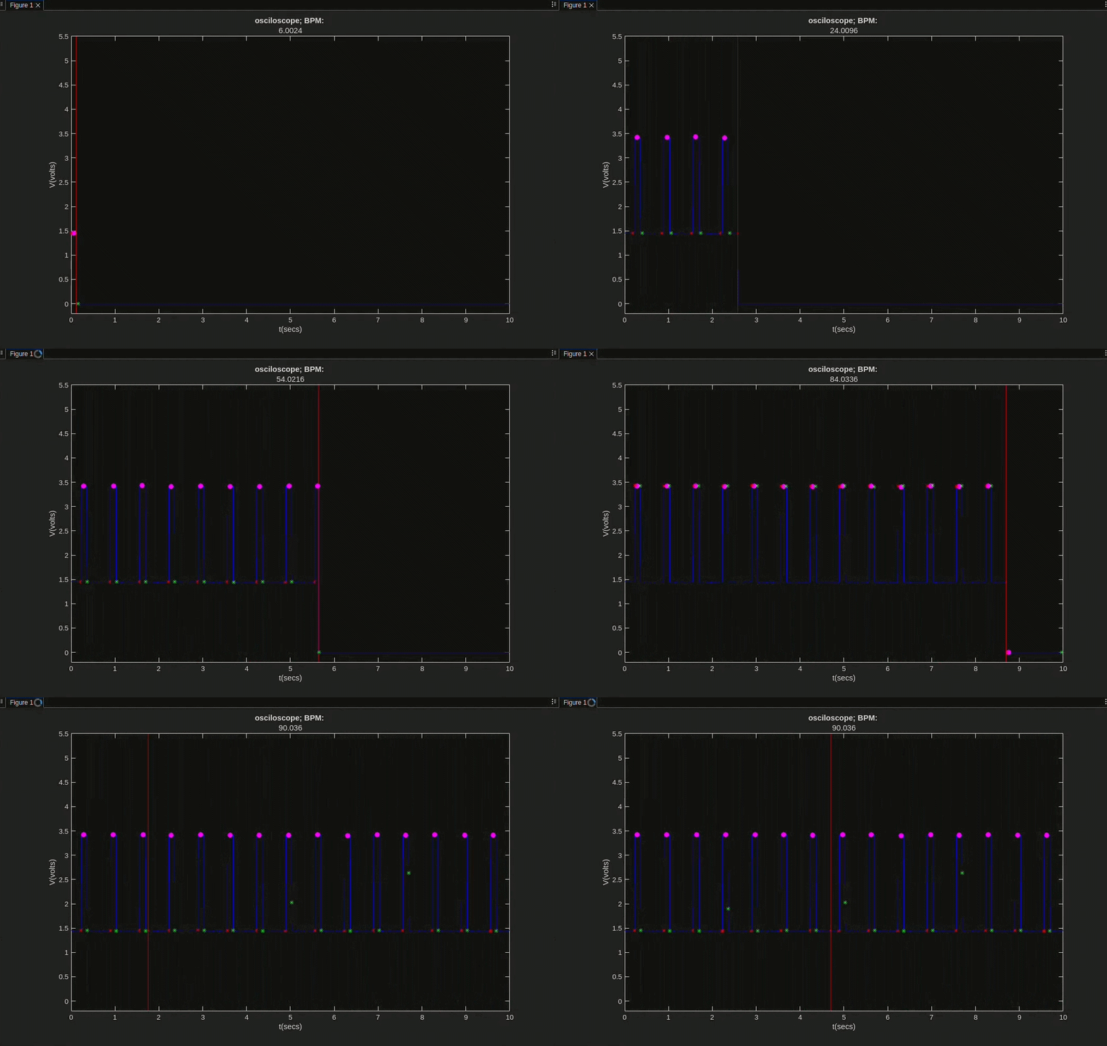
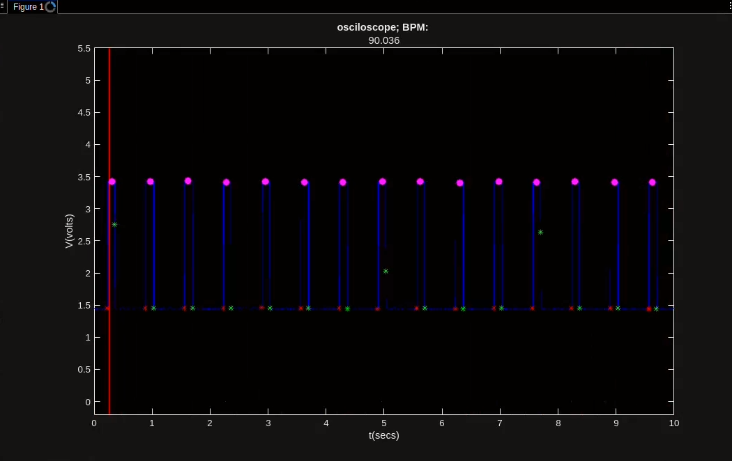
Figure 6: The image from the MATLAB srcipt running that shows the BPM of the signal, which is around 90 times a second for a minute, or around 1.5Hz.
While the BPM can be seen in Figure 3, it is shown again ib Figure 6. The BPM can be seen as 90, or 1.5Hz, which lines up with how the function generator was set up to output. This shows that the BPM calculation, and the software side of the ECG circuit as a whole, is working as intended.
Connecting the Hardware and Software
Results
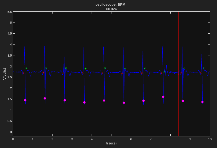
Figure 7: The image from the MATLAB srcipt running that shows the BPM of the generated heartbeat signal, which is around 60 times per minute, or around 1Hz.
Once the circuit board was connected to the Arduino or MATLAB, and the output from Figure 7 with the same BPM as generated from the heartbeat signal generator, it shows that the system works. Despite the little hiccup of the R location marker where the marker is on the lower S spike instead of the R peak, the count of the BPM and the output of the entire system is correct and show that everything works.
Conclusion and Future Work
With the overall results of the completed hardware and software integration showing that the accurate heartbeat shape normalized in between 0 and 5V and counting same BPM value that the heartbeat device, it is safe to say that the overall circuit works. Every apsect does what it is supposed to do, despite some flaws.
The main issues that were had with the ECG circuit as a whole was the slow speed of the "real-time" system and the fact that the MATLAB script counts the bottom part of the QRS complex instead of the R peak like it should. The slow "real-time" data collection issue can be solved with a faster, more powerful computer. The R peak detection, on the other hand, is due to the fact that the heartbeat signal generator isn't completely accurate to an actual heartbeat. An actual heartbeat looks more like the image from Figure 1, with the S peak in the QRS complex being nowhere as large as what the heartbeat generator outputs in normal heartbeats. While most ECG images do look like Figure 1, there are some situations, either with abnormal heartbeats or with the placements of the electrodes [5, 6], a large S peak can occur and have a larger value than the R peak. Due to this oversight in assumption of the QRS complex that has then bleed into the Code Snipet 2 with the 'identityQRSComplex' function, a fix that needs to not only look into the value of the peak but into the positive value while having better checks with the Q and S peaks to better mark on the plot of the signal would be the next step to take. But other than that, this combination of hardware signal detection, filtering, and normalization to software real-time QRS complex detection and BPM calculation works overall.
Due to manufacturing error, the circuit was not completely implemented at the time of this report. Future steps in this reguard are to fix the milling machine by replacing the bits, milling out the PCB, soldering the components, and testing the circuit as related in the testing portion of this report. The hardware and software when both verified to be working will be combined to a full implementation, and the further software implementations will be added.
[3] Jaakko Malmivuo and R. Plonsey, Bioelectromagnetism : Principles and Applications of Bioelectric and Biomagnetic Fields. New York Oxford University Press -10-05, 1995.
This signal of the heartbeat, in the form of the "PQRST" complex as seen with Figure 1, is what needs to be detected in order to find important information about a patient's heart.
Single-channel surface-EMG front end (AD623 + driven-right-leg) on a Raspberry Pi Pico. Board fabricated and telemetry verified on hardware; analog front end and on-body EMG still in bring-up.
It measures 66.5 × 53 mm and has 2 copper layers, 1.6 mm thick.
What parts does the ECG Project Josh use?
35 parts, built around the AD623AN. The full list of its parts is on this page, with links to each part's symbol and footprint where PCBKit's library has them.
Where can I download the ECG Project Josh KiCad files?
From the TallesSantosCUBoulder/ECEN4532_DSPLab_Spring2026_ECG_Project repository on GitHub, at the commit this page was made from: the board is ECG_KICAD_Files/ECG_Project_Josh_Emilie/ECG_Project_Josh.kicad_pcb and its schematic ECG_KICAD_Files/ECG_Project_Josh_Emilie/ECG_Project_Josh.kicad_sch. PCBKit opens the board in the browser, with nothing to install.
Can I use the ECG Project Josh design in my own project?
Its repository publishes it under the MIT licence: you may reuse it on that licence's terms (keep the author's notice, and for a copyleft licence share your changes alike).


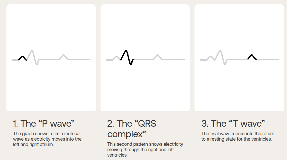 Figure 1: A diagram of the different parts of a heartbeat that are searched for during an ECG test [2].