2 layers107.6 × 45.1 mm
CTL-6.1
mekanii/ESU
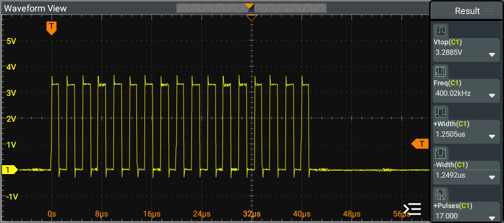
Below is the output scope from the sense circuit, where the pad resistance values are 5Ω, 200Ω, 1kΩ, and High Impedance.
80 parts

 mekanii/ESU
Below is the output scope from the sense circuit, where the pad resistance values are 5Ω, 200Ω, 1kΩ, and High Impedance.
RLoad is an open-source printed circuit board by mekanii, from the mekanii/ESU repository on GitHub. It is a 2-layer board of 179.1 × 88.9 mm with 100 parts on 92 nets.
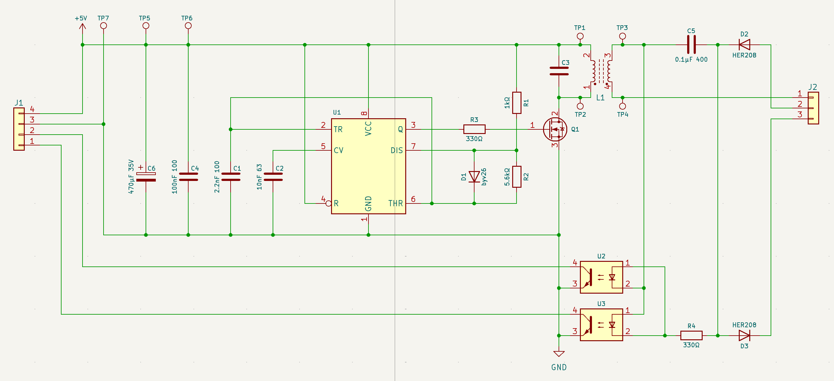

Below is the output scope at the input and output of toroidal transformer.

[!NOTE] All measurements for Return Electrode Monitoring do not utilize a physical Return Electrode; instead, a variable resistor is used. Therefore, all references to pad resistance in this context describe the variable resistor that simulates the Return Electrode.
Below is the output scope from the sense circuit, where the pad resistance values are 5Ω, 200Ω, 1kΩ, and High Impedance. The voltages measured by the oscilloscope are 10.385 mV, 558.91 mV, 689.31 mV, and 1.1164 V, respectively.

The ESP32's ADC provides a versatile and powerful way to read analog signals with a resolution of up to 12 bits and operates with a reference voltage of 0V to 3.3V (the default voltage range). Below is the formula to calculate the voltage per level for the ADC at 12-bit resolution.
$Voltage \ per \ Level = \frac{Voltage \ Range}{2^{Resolution}} = \frac{3.3V - 0V}{2^{12}} = \frac{3.3V}{4096} ≈ 0.00080586V ≈ 0.80586 mV$
Below is the formula to calculate the ADC value based on the voltage sense and the Voltage per Level.
$ADC \ Value = \frac{V_{sense}}{Voltage \ per \ Level}$
Using the formula above, we have the following ADC values for different pad resistances:
| Pad Resistance | Measured Voltage | ADC Value |
|---|---|---|
| 5Ω | 10.385 mV | 19 |
| 200Ω | 558.91 mV | 694 |
| 1kΩ | 689.31 mV | 855 |
| High-Z | 1116.4 mV | 1385 |
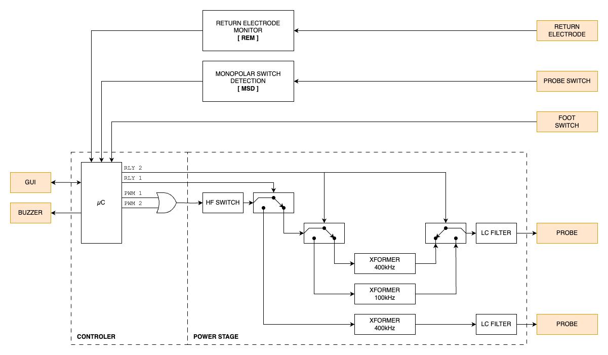
The Remote Control Module (RMT) on the ESP32 is a versatile hardware peripheral designed primarily for sending and receiving infrared signals. However, it can also be effectively utilized to generate precise Pulse Width Modulation (PWM) signals.
The clock divider is a crucial parameter in microcontroller and digital circuit design that determines the frequency of a clock signal by dividing the input clock frequency, which is APB_CLK (80 MHz) for ESP32.
$Clock \ Divider = \frac{APB _ CLK}{Clock \ Frequency}$
The resolution in duty cycle is a crucial parameter in microcontroller and digital circuit design that determines the granularity of control over the PWM signal. It defines how finely the duty cycle can be adjusted, allowing for precise modulation of the output signal. In the case of the ESP32, the resolution is influenced by the clock frequency which ultimately affect the ability to achieve desired output levels.
$Resolution = \frac{Clock \ Frequency}{PWM \ Frequency}$
The combination of clock frequency and resolution plays a vital role in determining the performance of PWM signals in microcontroller applications. The clock frequency sets the base rate at which the system operates, while the resolution defines how many discrete levels the duty cycle can be divided into. A higher clock frequency allows for faster switching and more precise timing, while a higher resolution enables finer control over the duty cycle. Together, they influence the accuracy and responsiveness of the PWM output, making it essential to balance these parameters to meet the specific requirements of the application.
| Mode | f PWM | f Clock | Clock Div | Resolution |
|---|---|---|---|---|
| Pure Cut | 400 kHz | 80 MHz | 1 | 200 |
| Blend Cut 1 | 400 kHz | 80 MHz | 1 | 200 |
| Blend Cut 2 | 400 kHz | 80 MHz | 1 | 200 |
| Coag Spray | 25 kHz | 10 MHz | 8 | 800 |
| Coag Forced | 20 kHz | 10 MHz | 8 | 1000 |
| Coag Standard | 400 kHz | 80 MHz | 1 | 200 |
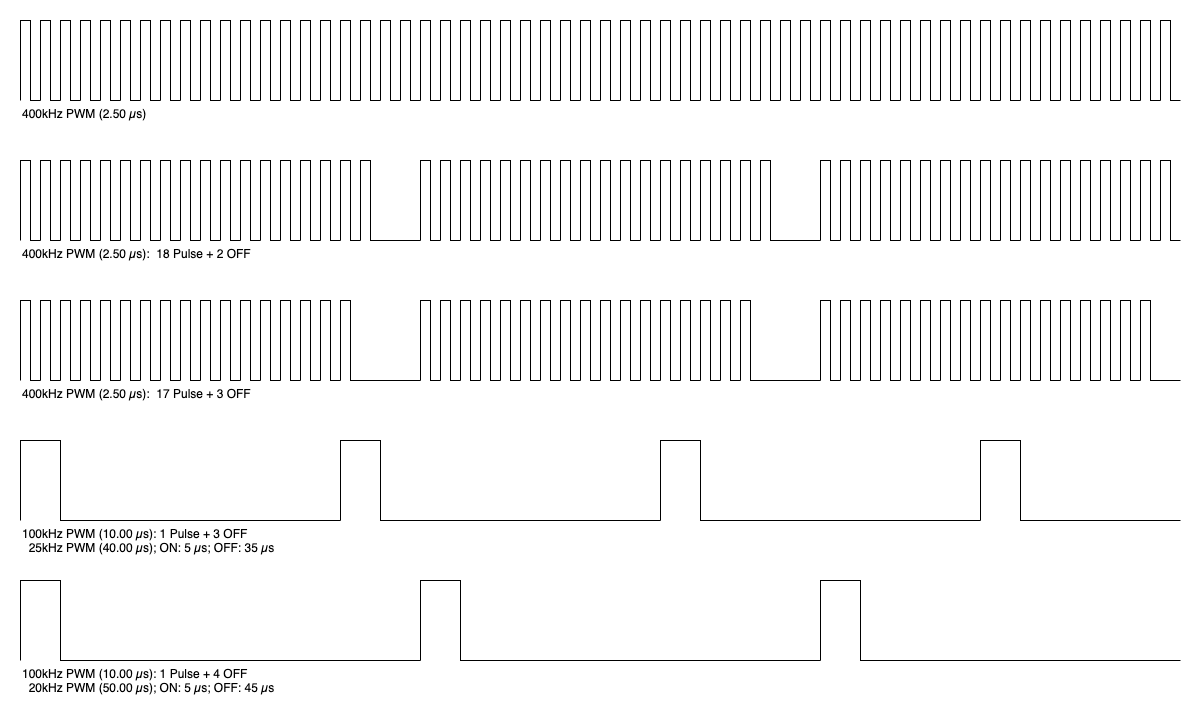
[!NOTE] 400kHz PWM signal utilize a discrete resolution of 200 levels.
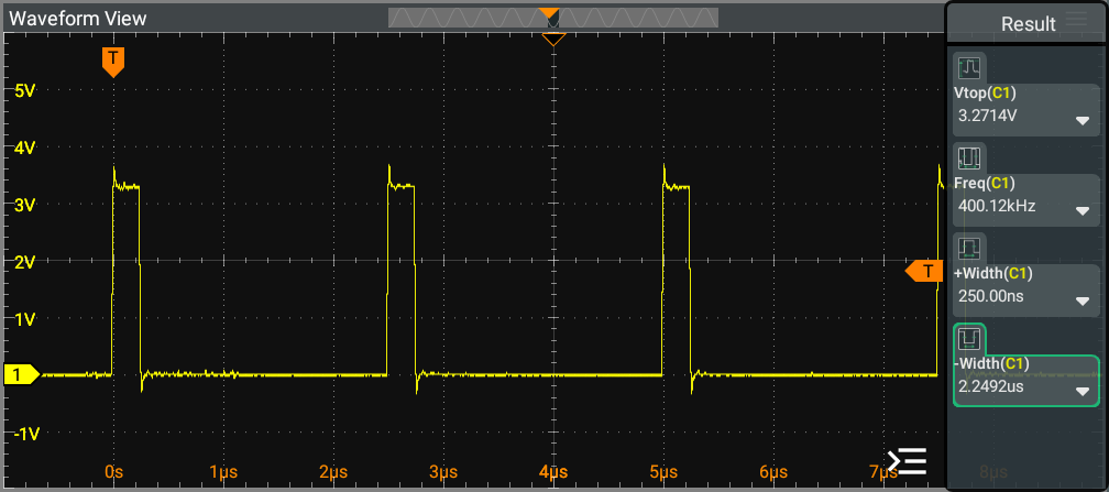
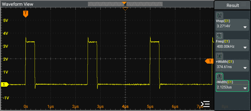
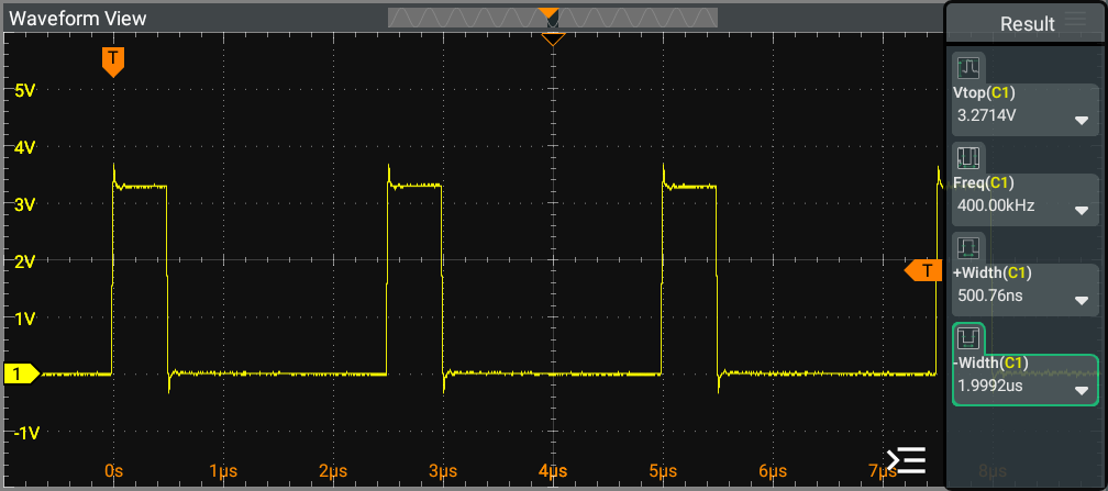
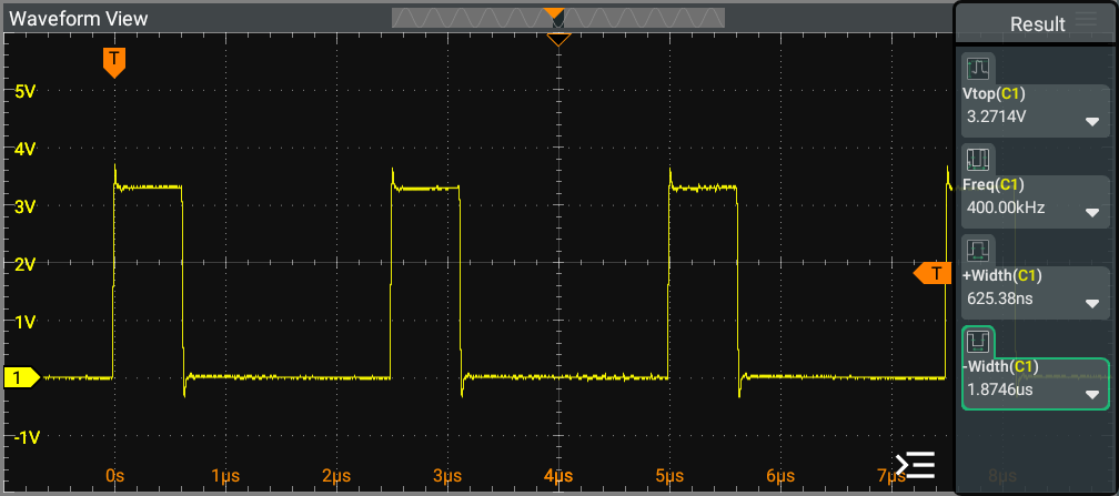
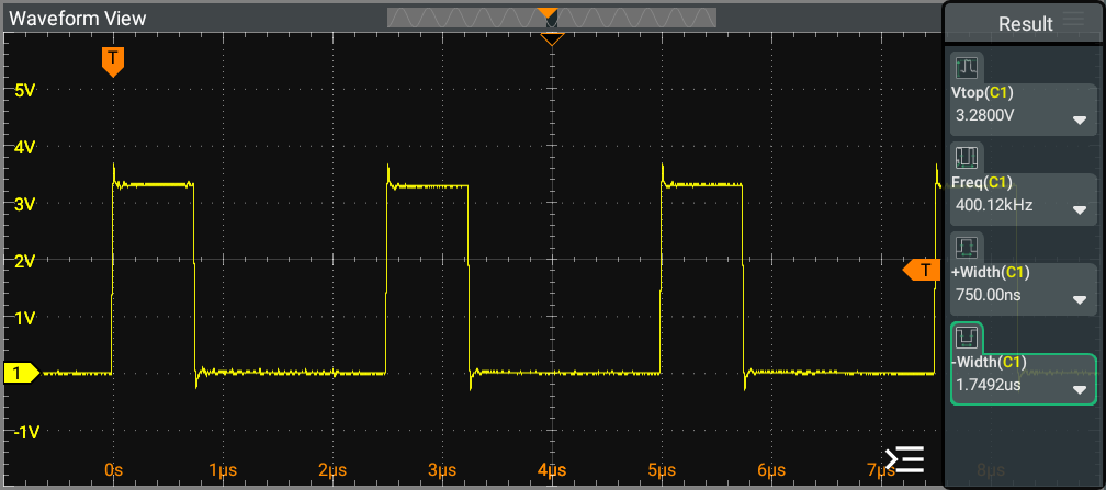
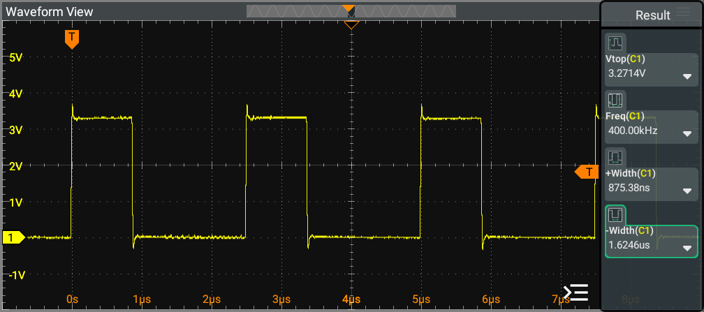
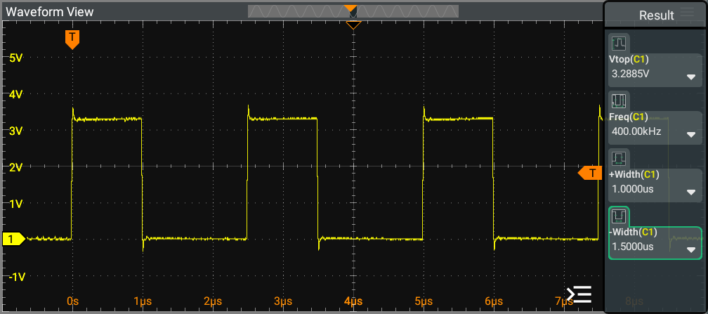
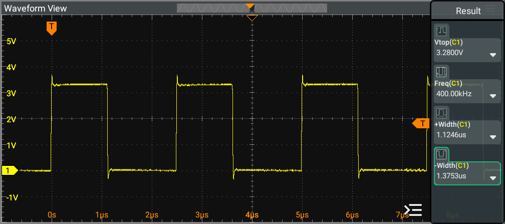
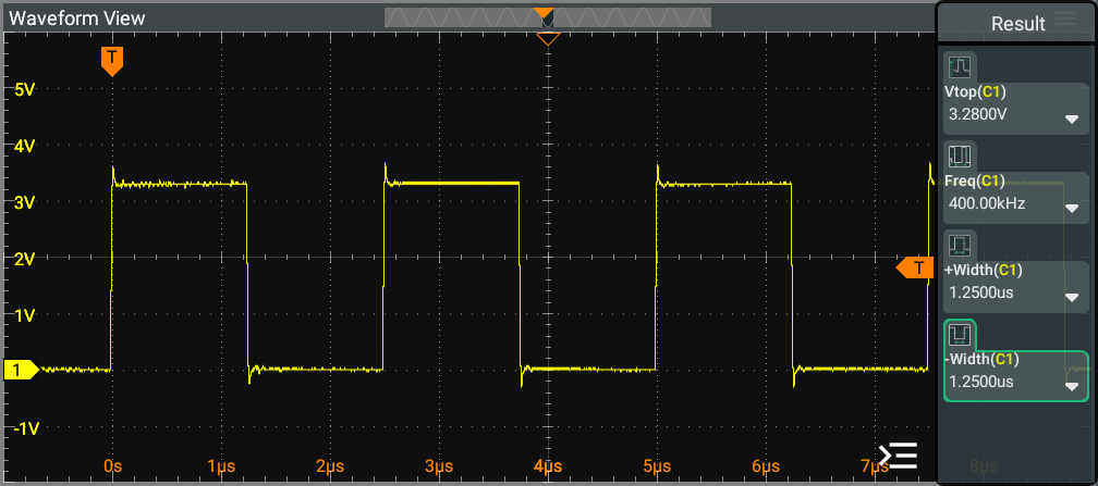
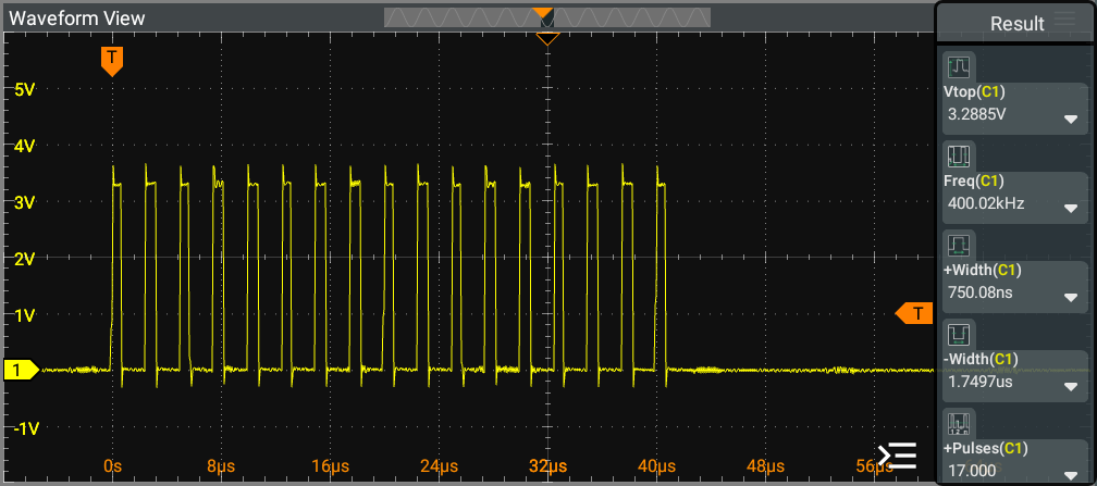
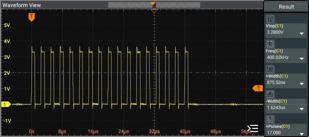
[!NOTE] Pattern 2: 18 pulses per 1 modulation (400 kHz for each pulse, with 0% PWM during the last 2 periods).
This pattern utilize a discrete resolution of 200 levels, similar to that of a Pattern 1 (Pure Cut) PWM signal.
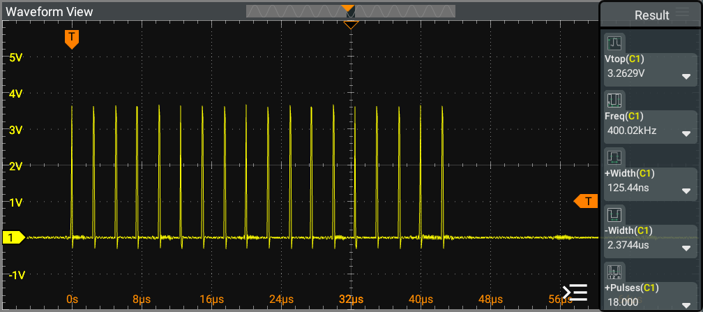
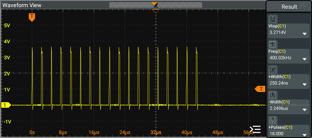
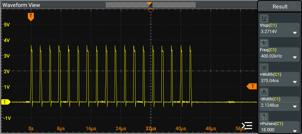
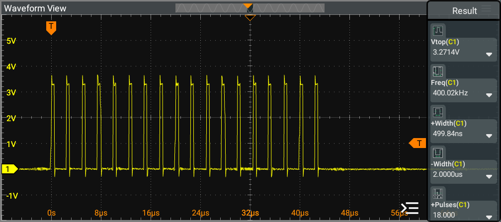
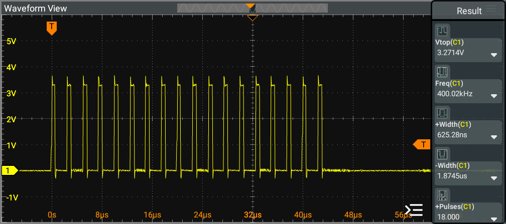
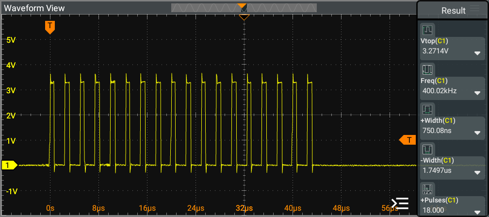
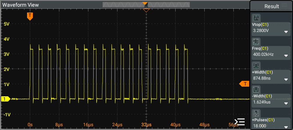
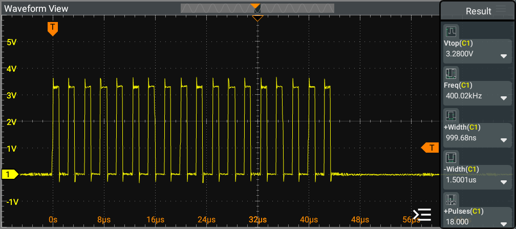
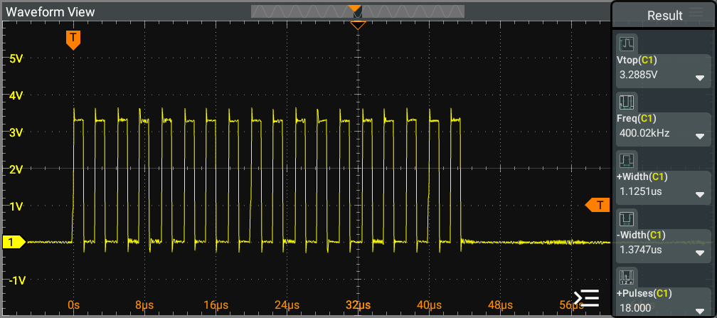
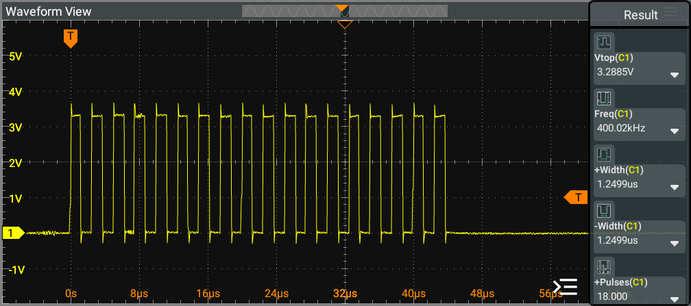
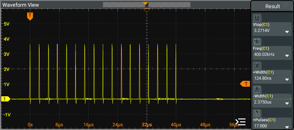
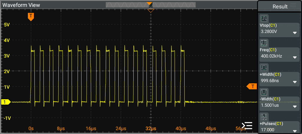
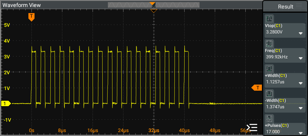
[!NOTE] Pattern 3: 17 pulses per 1 modulation (400 kHz for each pulse, with 0% PWM during the last 3 periods).
This pattern utilize a discrete resolution of 200 levels, similar to that of a Pattern 1 (Pure Cut) PWM signal.
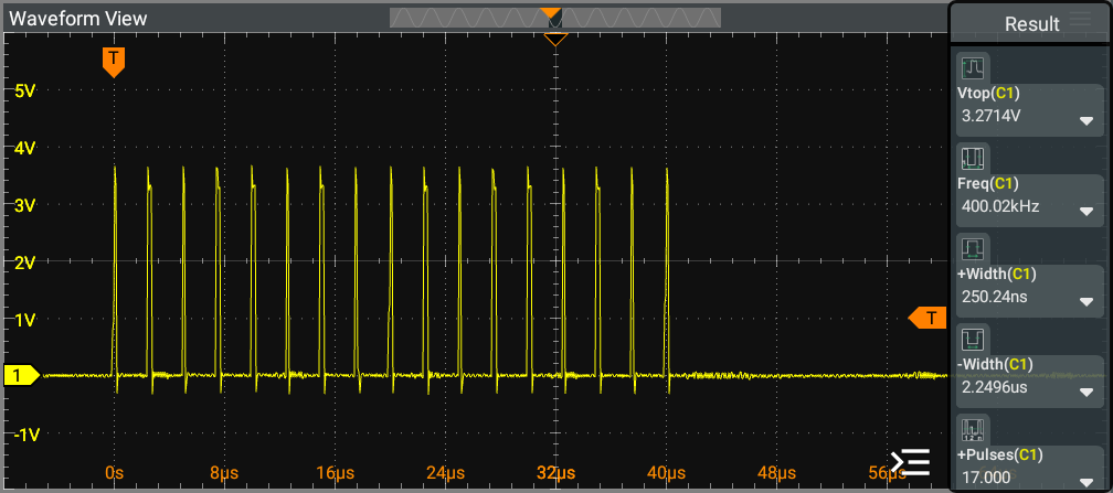
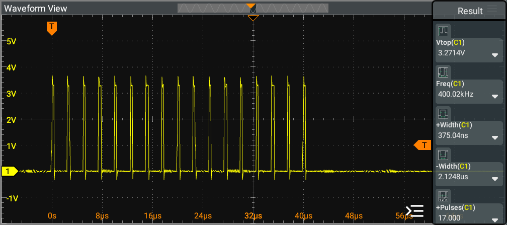
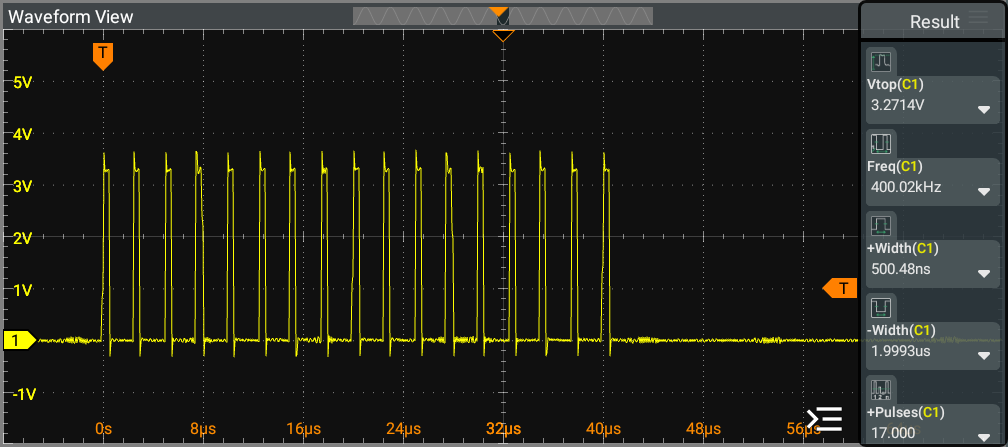
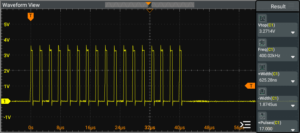
The image illustrates the output scope for the 25kHz (Spray Coagulation operation) at the PWM generator. It provides a detailed view of the waveform characteristics and performance metrics associated with the Spray Coagulation process, highlighting the key features and behavior of the PWM signal during this operation.
For discrete levels ranging from 10 to 100, demonstrates similar PWM frequency, indicating consistent performance across these duty cycle settings. We can observe that the increment of the duty cycle results in a pulse that exhibits a linear increase in HIGH time, further emphasizing the effectiveness of the PWM modulation in maintaining a predictable response across varying duty cycle levels.
[!NOTE] 25kHz PWM signal utilize a discrete resolution of 800 levels.
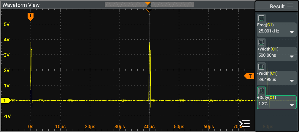
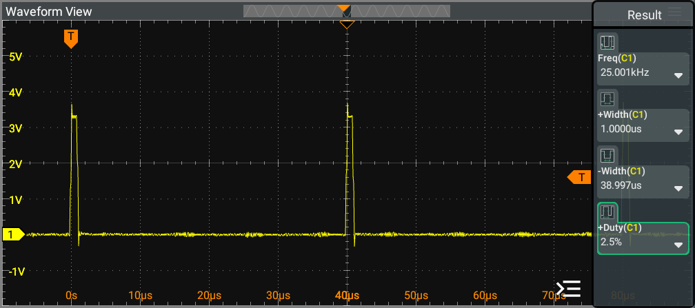
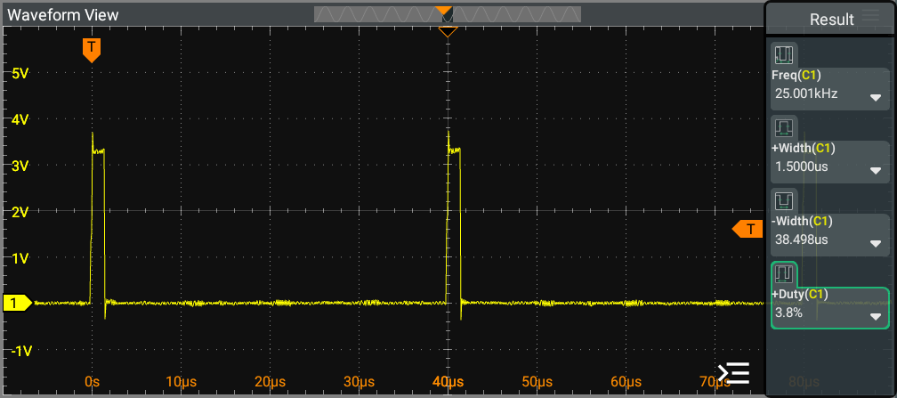
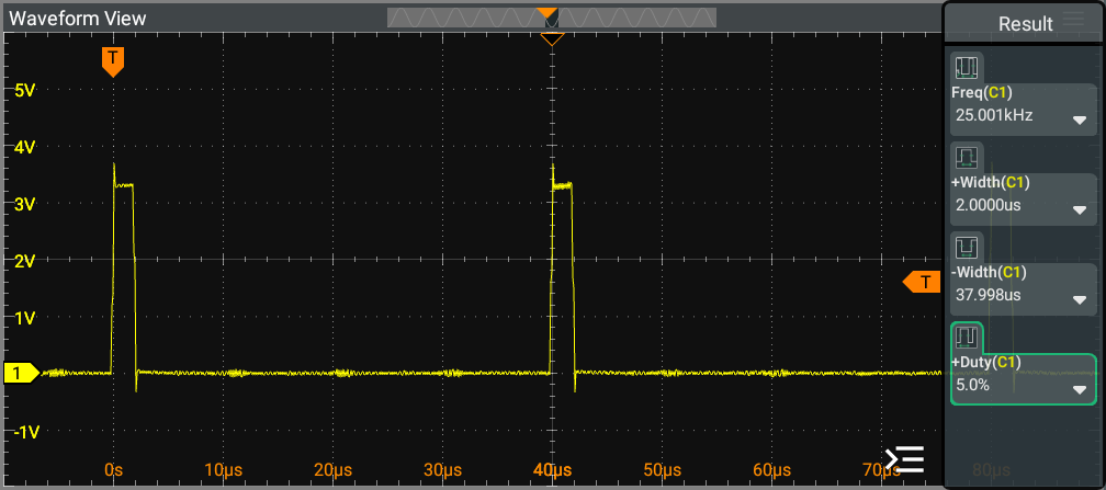
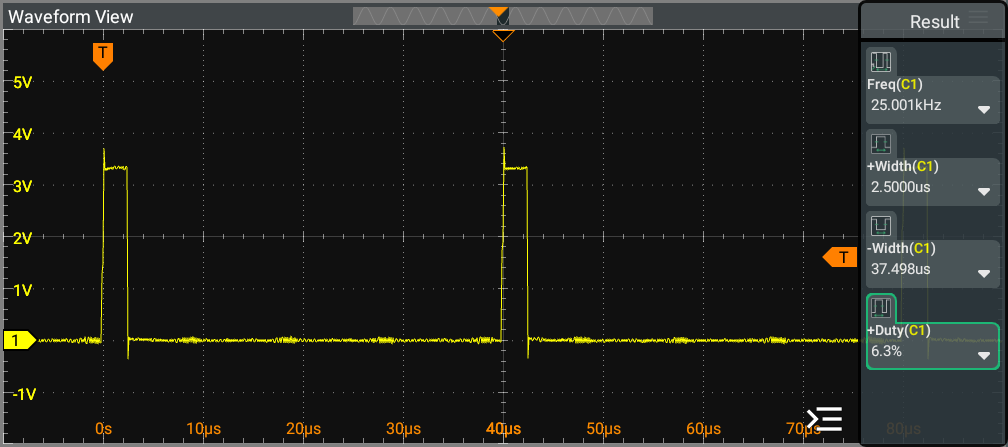
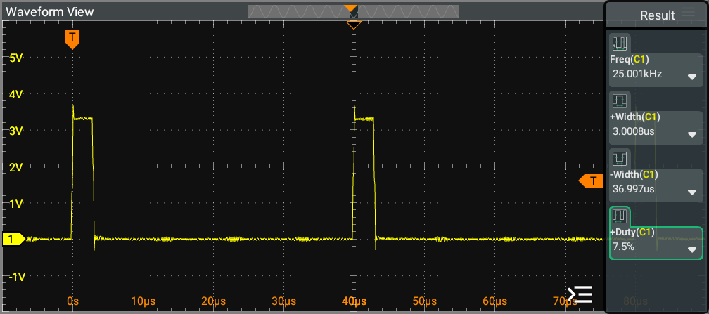
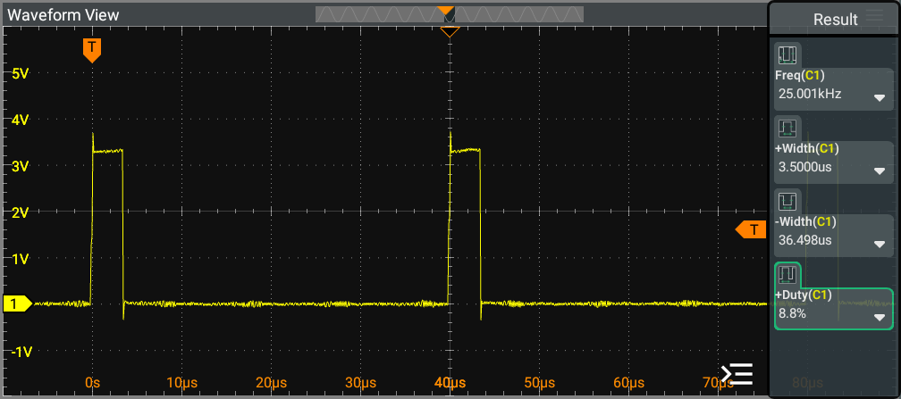
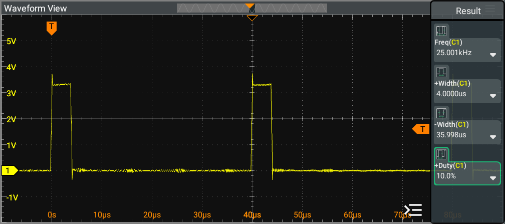
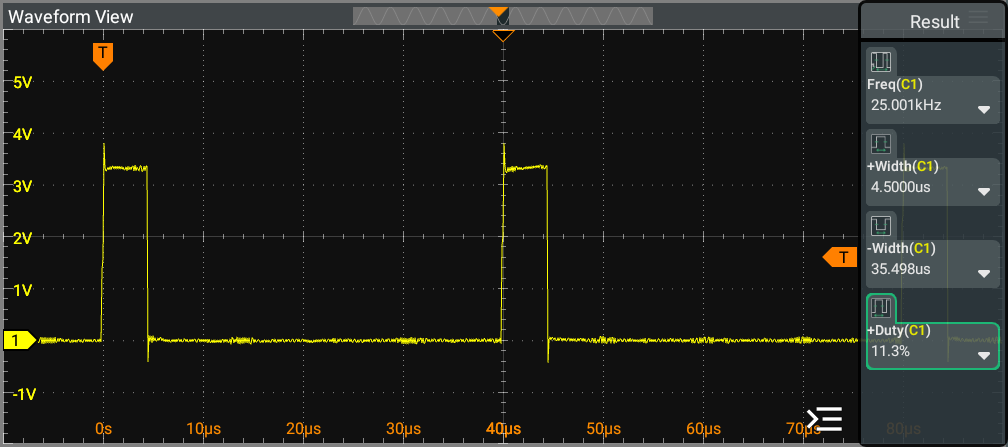
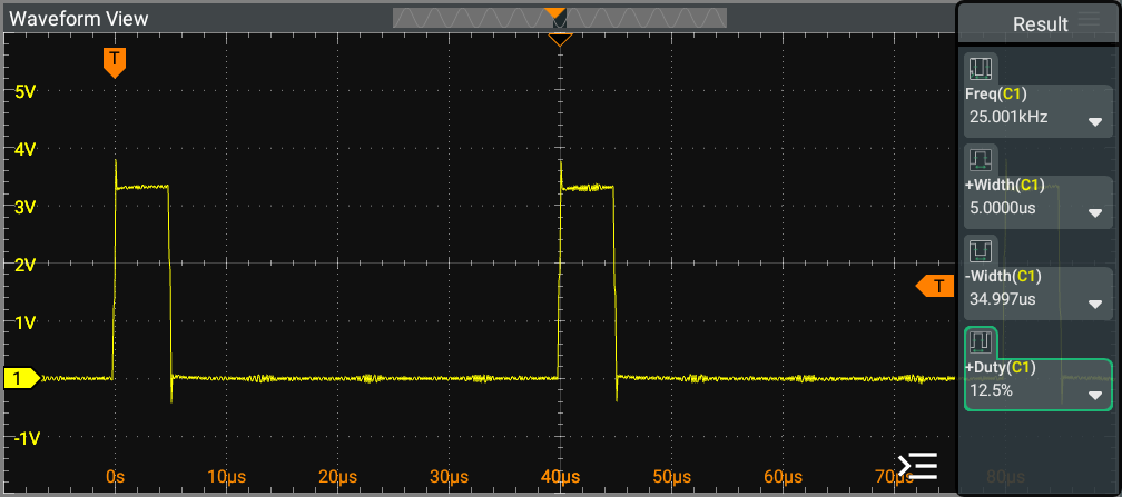
| Discrete Level | Duty Cycle | HIGH Time | LOW Time |
|---|---|---|---|
| 10 | 1.25 % | 0.5 µs | 39.5 µs |
| 20 | 2.50 % | 1.0 µs | 39.0 µs |
| 30 | 3.75 % | 1.5 µs | 38.5 µs |
| 40 | 5.00 % | 2.0 µs | 38.0 µs |
| 50 | 6.25 % | 2.5 µs | 37.5 µs |
| 60 | 7.50 % | 3.0 µs | 37.0 µs |
| 70 | 8.75 % | 3.5 µs | 36.5 µs |
| 80 | 10.00 % | 4.0 µs | 36.0 µs |
| 90 | 11.25 % | 4.5 µs | 35.5 µs |
| 100 | 12.50 % | 5.0 µs | 35.0 µs |
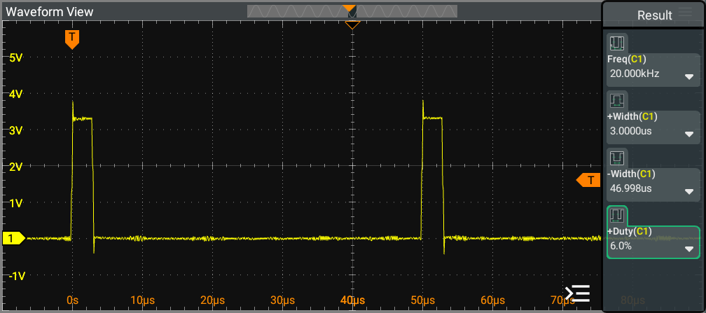
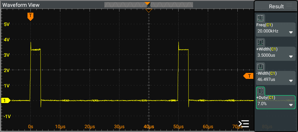
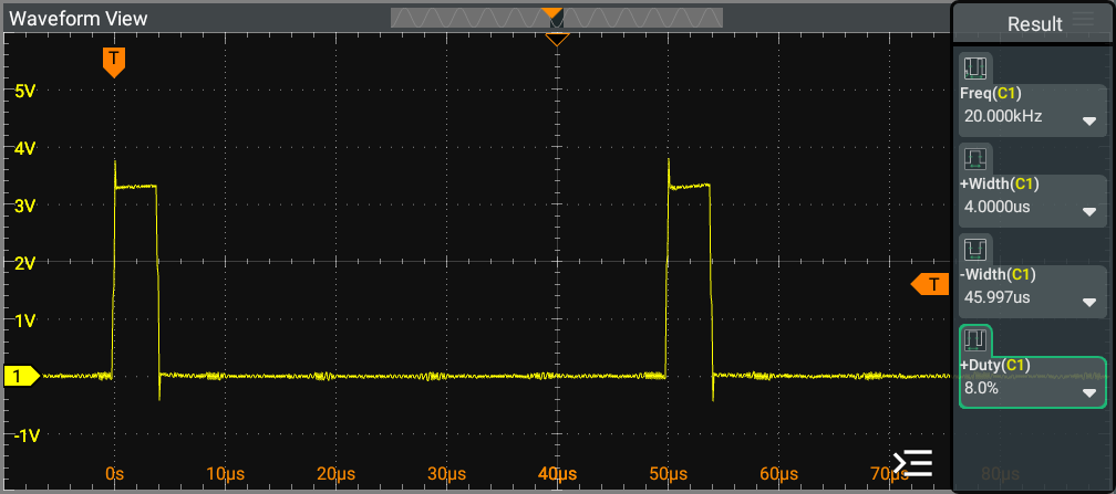
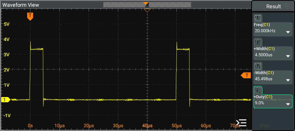
The image illustrates the output scope for the 20kHz (Forced Coagulation operation) at the PWM generator. It provides a detailed view of the waveform characteristics and performance metrics associated with the Forced Coagulation process, highlighting the key features and behavior of the PWM signal during this operation.
For discrete levels ranging from 10 to 100, demonstrates similar PWM frequency, indicating consistent performance across these duty cycle settings. We can observe that the increment of the duty cycle results in a pulse that exhibits a linear increase in HIGH time, further emphasizing the effectiveness of the PWM modulation in maintaining a predictable response across varying duty cycle levels.
[!NOTE] 20kHz PWM signal utilize a discrete resolution of 1000 levels.
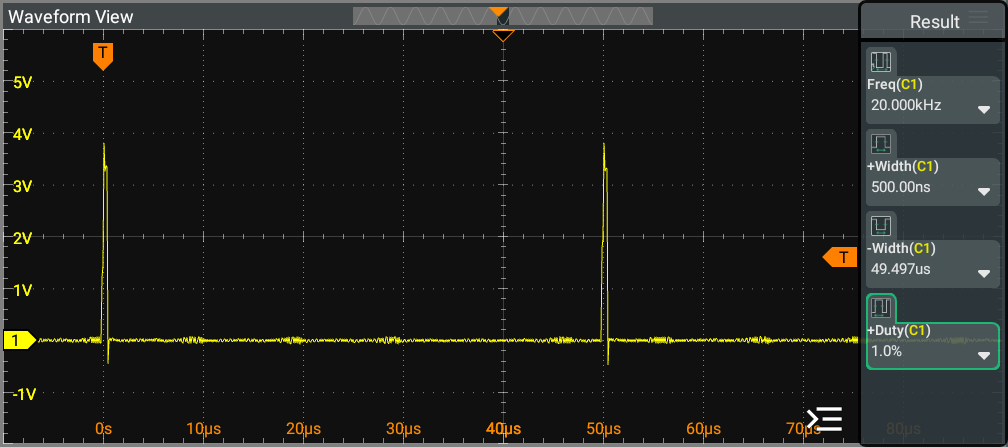
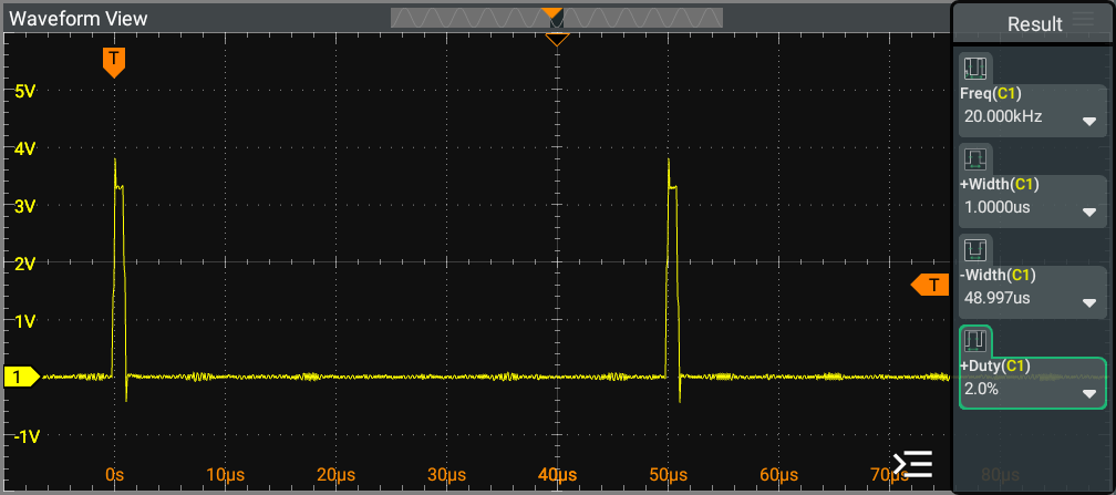
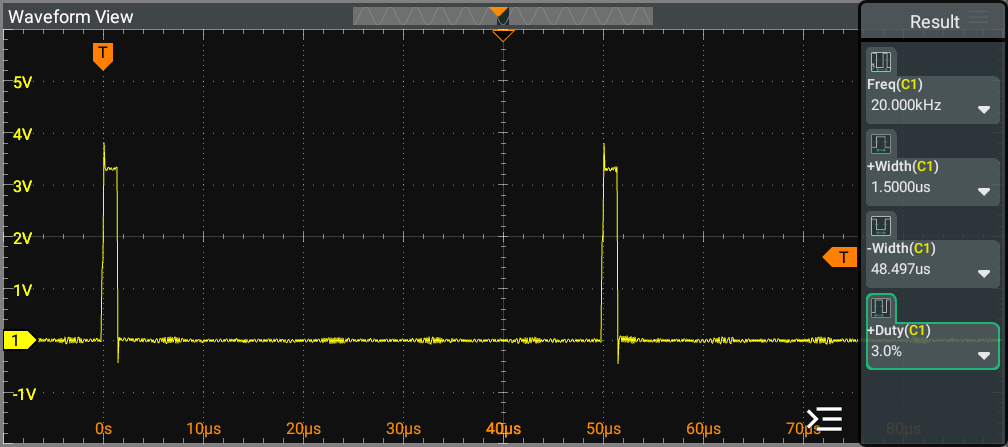
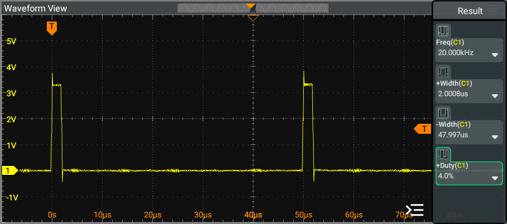
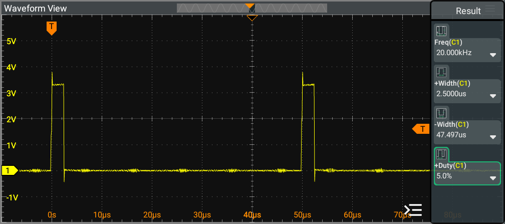
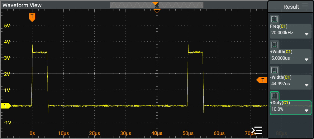
| Discrete Level | Duty Cycle | HIGH Time | LOW Time |
|---|---|---|---|
| 10 | 1.00 % | 0.5 µs | 49.5 µs |
| 20 | 2.00 % | 1.0 µs | 49.0 µs |
| 30 | 3.00 % | 1.5 µs | 48.5 µs |
| 40 | 4.00 % | 2.0 µs | 48.0 µs |
| 50 | 5.00 % | 2.5 µs | 47.5 µs |
| 60 | 6.00 % | 3.0 µs | 47.0 µs |
| 70 | 7.00 % | 3.5 µs | 46.5 µs |
| 80 | 8.00 % | 4.0 µs | 46.0 µs |
| 90 | 9.00 % | 4.5 µs | 45.5 µs |
| 100 | 10.00 % | 5.0 µs | 45.0 µs |
The system UART mode is fixed to 8N1, and the baud rate is 115200.
Frame Structure
The data frame consists of 5 data blocks:
[HEADER] [LENGTH] [INSTRUCTION] [PAYLOAD] [CRC]
Frame Components
| Block | Size [byte] | Description | Value |
| HEADER | 2 | Frame start marker | 0x5A 0XA5 |
| LENGTH | 1 | Total bytes after HEADER | INSTRUCTION + DATA + CRC |
| INSTRUCTION | 1 | Instruction Code | 0x82 : Write 0x83 : Read |
| PAYLOAD | 0 - 3 | Payload data | |
| CRC | 2 | Cyclic Redundancy Check |
The PAYLOAD frame consist 3 data blocks:
[VP ADDRESS] [NUMBER OF WORDS] [DATA]
| Block | Size [byte] | Description |
| VP ADDRESS | 2 | Variable Pointer address to read from |
| NUMBER OF WORDS | 1 | Number of data words to read (always 1) |
| DATA | 2 | Data word read from the specified VP address |
| Command | Variable | VP ADDRESS | INSTRUCTION | Data Frame | Response |
| System status query | | | | | |
| System reset | | | | | |
| Stop all RMT transmission | | | | |
| Command | Variable | VP ADDRESS | INSTRUCTION | Data Frame | DATA | Response |
| Get/set mode selection Cut | | | | |
| |
| Get/set mode selection Coag | | | | |
|
| Command | Variable | VP ADDRESS | INSTRUCTION | Data Frame | DATA | Response |
| Get/set discrete level 400kHz - Pattern 1 | | | | | | |
| Get/set discrete level 400kHz - Pattern 2 | | | | | | |
| Get/set discrete level 400kHz - Pattern 3 | | | | | | |
| Get/set discrete level 25kHz | | | | | | |
| Get/set discrete level 20kHz | | | | | | |
| Get/set discrete level 400kHz - Bipolar Standard | | | | | |
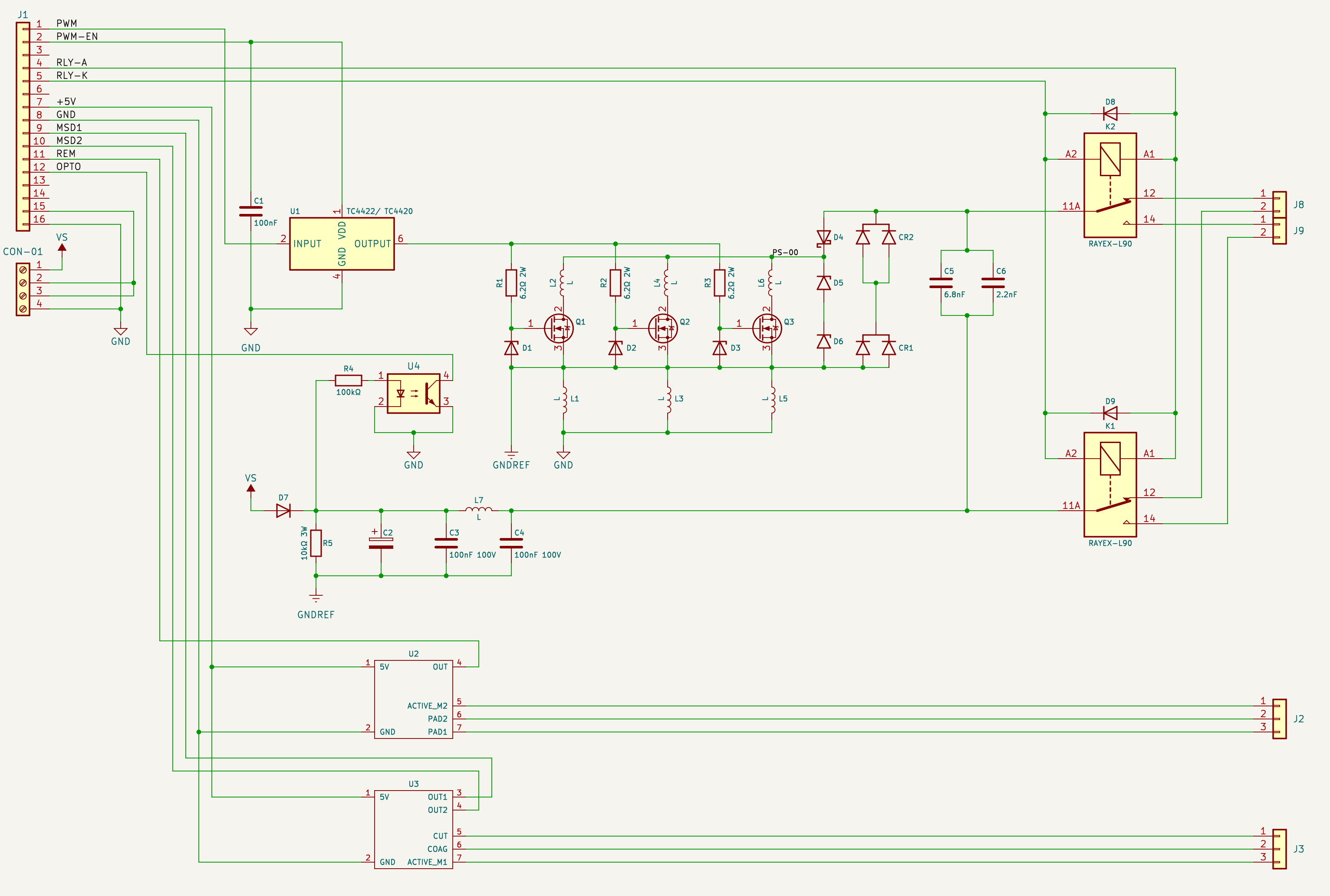
We use the TC4420 as our MOSFET driver due to its high-speed performance and ability to efficiently drive N-channel MOSFETs in various applications. The TC4420 provides a peak output current of up to 6A, allowing for rapid charging and discharging of the MOSFET gate capacitance. This capability minimizes switching losses and enhances overall efficiency in power management.
Operating within a supply voltage range of 4.5V to 18V, the TC4420 can effectively drive MOSFET gates at a voltage level of 12V, ensuring that the MOSFET turns on fully for optimal performance. Its fast switching speed, with propagation delays in the nanosecond range (typically 55ns), is crucial for high-frequency applications, reducing transition times and heat generation.
We use three IRFPE50 MOSFETs in parallel to enhance the overall performance and reliability of our circuit. The decision to parallel these MOSFETs is driven by several key factors:
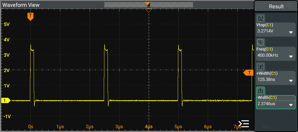
The image illustrates the output scope for the 400kHz operation at:
It provides a detailed view of the waveform characteristics and performance metrics associated with the Pure Cut process, highlighting the key features and behavior of the HF Switch signal during this operation.
For discrete levels ranging from 20 to 180, demonstrates similar Waveform frequency, indicating consistent performance across these duty cycle settings.
[!NOTE] 400kHz PWM signal utilize a discrete resolution of 200 levels.
Toroidal Ferrite Core Transformer
A toroidal ferrite core transformer is a type of transformer that uses a ring-shaped (toroidal) core made from ferrite material. Ferrite is a ceramic compound consisting of iron oxide mixed with other metals, which provides high magnetic permeability and low electrical conductivity. This makes ferrite ideal for high-frequency transformer applications.
Structure and Construction
Key Advantages
Power Handling
The transformer’s power rating is determined by the product of output voltage and current, and the core must be sized to avoid saturation at maximum load.
Skin Effect
At high frequencies, the skin effect is a phenomenon in alternating current (AC) where the current density becomes highest at the surface of a conductor and decreases exponentially toward the center. This occurs because the alternating current generates a changing magnetic field, which in turn induces eddy currents within the conductor. These eddy currents oppose the main current flow more strongly at the center, forcing most of the AC current to flow near the surface. As a result, the effective cross-sectional area available for current flow is reduced, increasing the effective resistance of the wire at higher frequencies.
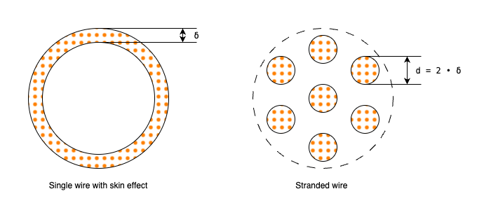
The depth at which the current density falls to 37% of its value at the surface.
$δ = \sqrt{ \frac{ ρ } { π • f • μ } }$
Where:
For high-frequency windings, consider using multiple thinner wires in parallel (Litz wire) to reduce skin effect losses.
The calculated diameter above is based on DC or low-frequency AC. For high-frequency applications, the effective area may be less than the physical area due to skin effect.
The effective cross-sectional area of the core is calculated as:
$A_e = \frac{( OD – ID ) • H }{ 2 }$
This area is important for determining how much magnetic flux the core can handle without saturating.
The number of primary turns is determined by:
$N_p = \frac{ V_{in} • Duty \ Cycle • 10^{10} }{ 2 • f • B_{max} • A_e }$
This ensures the core does not saturate at the maximum input voltage and duty cycle.
The voltage induced per turn is:
$Volt \ per \ turn = \frac{ V_{in} }{ N_p }$
The number of secondary turns is:
$N_s = \frac{ V_{out} }{ Volt \ per \ turn }$
This ensures the transformer provides the correct output voltage.
$P = V_{out} • I_{out}$
$I_{in} = \frac{ P }{ V_{in} }$
These calculations confirm the input current required to deliver the desired output power.
For high-frequency applications, we need to consider:
To calculate the required wire diameter for a given current, use the formula:
$dW = \sqrt{ \frac{ 4 • I }{ \pi • J } }$
Where:
The skin depth in copper is approximately calculated by following formula:
$δ = \sqrt{ \frac{ ρ } { π • f • μ } }$
If our calculated wire diameters are larger than 2× skin depth, consider using:
Required copper area is the net copper cross‑section needed to carry the target current without exceeding your thermal/current‑density limit. Pick $J$ based on allowed temperature rise and cooling. Typical transformer design uses $J=1.5$–$3.0$ A/mm²; choose the lower end for continuous duty, compact windings, or poor airflow; higher values may be acceptable for pulsed or well‑cooled designs.
$A_{req} = \frac{I}{J}$
Area per strand is the metallic copper area of a single strand. Use the bare copper diameter (exclude enamel). If you only have an enamelled wire gauge, subtract twice the enamel thickness to estimate bare diameter, or use datasheet bare area.
$A_{strand} = \frac{pi • d_{strand}^2}{4}$
Number of strands is calculated by following formula
$N_{strands} = ⌈ \frac{A_{req}}{A_{strand} • η_{pack}} ⌉$
Where:
Length per turn (mean path around toroid)
$Length \ per \ turn = 2 • (\frac{OD - ID}{2} + H)$
Individual conductor length (per strand, includes ~10% leads allowance):
$Individual \ Length = 1.1 • N • Length \ per \ turn$
Total copper length for the bundle (all parallel strands combined):
$Total \ Length = N_{strands} • Individual \ Length$
$Total \ Wire \ Length \ Needed = Total \ Length_{\ p} + Total \ Length_{\ s}$
| $f$ [Hz] | $V_{in}$ [V] | $V_{out}$ [V] | $I_{out}$ [A] | $P$ [W] | $I_{in}$ [A] | $ID$ [mm] | $OD$ [mm] | $H$ [mm] | $A_e$ [mm²] | $B_{max}$ [Gauss] | $N_p$ [turns] | $Volt \ per \ turn$ [V/turn] | $N_s$ [turns] | $J$ [A/mm²] | $dW_p$ [mm] | $dW_s$ [mm] | $δ$ [mm] | $d_{p \ strand}$ [mm] | $d_{s \ strand}$ [mm] | $N_{p \ strands}$ | $N_{s \ strands}$ | $Individual \ Length_{\ p}$ [m] | $Total \ Length_{\ p}$ [m] | $Individual \ Length_{\ s}$ [m] | $Total \ Length_{\ s}$ [m] |
|---|---|---|---|---|---|---|---|---|---|---|---|---|---|---|---|---|---|---|---|---|---|---|---|---|---|
| 400,000 | 72 | 216 | 0.5 | 108 | 1.5 | 23.3 | 40.4 | 15.1 | 129.1 | 350 | 10 | 7.2 | 30 | 1.5 | 1.13 | 0.65 | 0.103 | 0.2 | 0.2 | 32 | 11 | 0.520 | 16.65 | 1.561 | 17.17 |
| 100,000 | 72 | 504 | 0.2 | 100 | 1.4 | 23.3 | 40.4 | 15.1 | 129.1 | 350 | 40 | 1.8 | 279 | 1.5 | 1.09 | 0.41 | 0.206 | 0.2 | 0.2 | 30 | 5 | 2.081 | 62.44 | 14.516 | 72.58 |
| 400,000 | 48 | 200 | 0.5 | 100 | 2.08 | 23.3 | 40.4 | 15.1 | 129.1 | 350 | 7 | 6.8 | 29 | 1.5 | 1.33 | 0.65 | 0.103 | 0.2 | 0.2 | 44 | 11 | 0.364 | 16.03 | 1.509 | 16.60 |
| 100,000 | 48 | 500 | 0.2 | 100 | 2.08 | 23.3 | 40.4 | 15.1 | 129.1 | 350 | 27 | 1.8 | 281 | 1.5 | 1.33 | 0.41 | 0.206 | 0.2 | 0.2 | 44 | 5 | 1.405 | 61.81 | 14.620 | 73.10 |
The image illustrates the output scope at output transformer 400kHz with PWM frequency 400kHz
For discrete levels ranging from 10 to 100, demonstrates similar Waveform length, indicating consistent performance across these duty cycle settings.
[!NOTE] 400kHz PWM signal utilize a discrete resolution of 200 levels.
The image illustrates the output scope at output transformer 100kHz with PWM frequency 25kHz
For discrete levels ranging from 10 to 100, demonstrates similar Waveform length, indicating consistent performance across these duty cycle settings.
[!NOTE] 25kHz PWM signal utilize a discrete resolution of 400 levels.
The image illustrates the output scope at output transformer 100kHz with PWM frequency 20kHz
For discrete levels ranging from 10 to 100, demonstrates similar Waveform length, indicating consistent performance across these duty cycle settings.
[!NOTE] 20kHz PWM signal utilize a discrete resolution of 500 levels.
Type 1 Butterworth Filter: Differential Filter
A Type 1 Butterworth filter is a second-order low-pass filter that provides a maximally flat frequency response in the passband. The "Type 1" designation typically refers to the specific topology or configuration of the filter circuit. In the context of differential filters, this often means a balanced configuration that processes differential signals (signals with equal and opposite components).
Differential Filter Configuration
A differential filter is designed to handle differential signals, which are commonly used in high-speed digital circuits, audio systems, and communication equipment. The filter processes both the positive and negative components of the signal simultaneously, providing better noise immunity and common-mode rejection.
Key Characteristics:
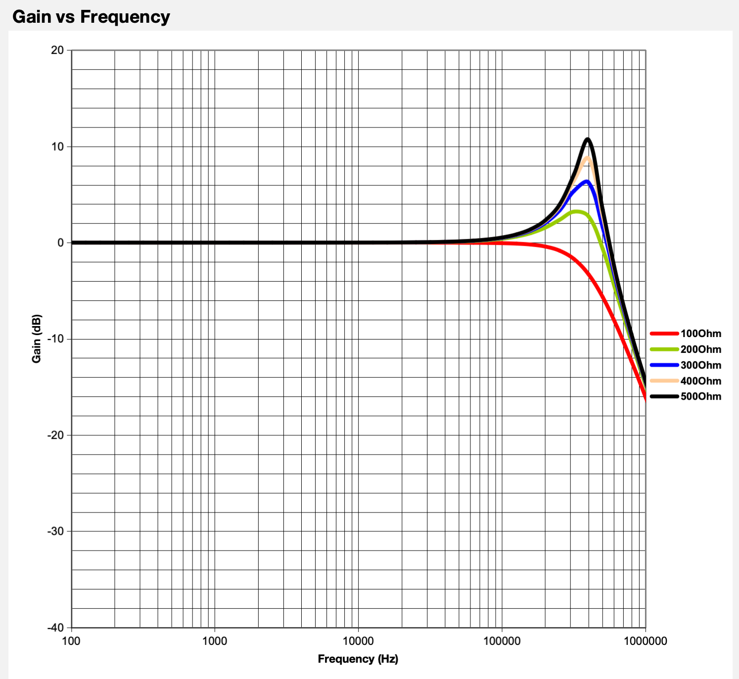
The frequency response of the second-order class-D LC output filter is critical when selecting the component values for the inductor and capacitor. The LC filter response also varies with load impedance. The load impedance determines the damping ratio of the output LC filter and is classified as:
It is also important to understand the load impedance variations for the application and select the L and C values that suit the expected load variations. Ideally, the LC filter value is selected for a critically damped, flat passband, and phase response. Two considerations when selecting components for the second-order low-pass filter is:
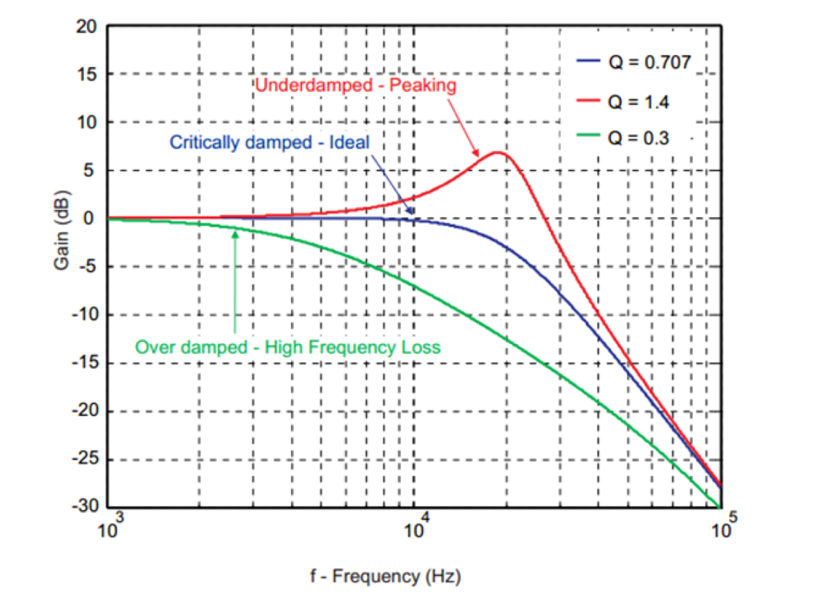
Texas Instrument recommends using a second-order Butterworth low-pass filter because of its flat pass-band and phase response. Texas Instrument does not recommend the use of LC filters that peak excessively, like the underdamped filter response shown in figure above. At high frequency, the peaks are generally harsh to the human ear and can also trigger the protection circuitry, such as overcurrent, of some amplifiers. However, overdamped filters result in attenuation of high-frequency signal content.
This section details the design and analysis of a Type 1 Butterworth Filter in single-ended LC circuit equivalent.
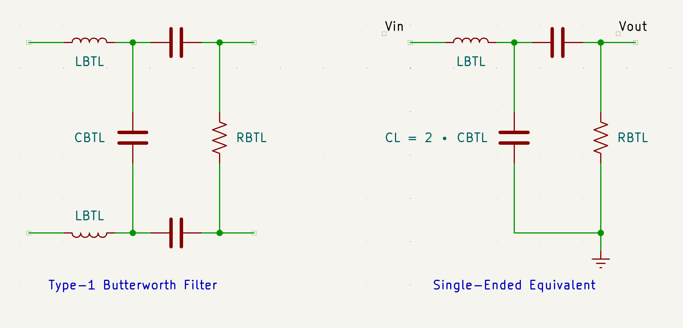
Cut-off Frequency for single-ended LC Filter
The cut-off frequency ($f_0$) of the LC filter is determined by the values of the inductor ($L_{BTL}$) and capacitor ($C_L$), using the formula:
$f_0 = \frac{ ⍵0 }{ 2 • π } = \frac{ 1 }{ 2 • π • \sqrt{ L{BTL} • C_L } }$
The quality factor ($Q$) describes the selectivity or sharpness of the filter’s response and is given by:
$Q = R_L • \sqrt{ \frac{ C_L }{ L_{BTL} } } $
where $R_L$ is the load resistance.
To design a filter that is critically damped with a Butterworth response, Q = 0.707 = 1/√2. By substituting Q = 1/√2 into equations for Cut-off Frequency and Quality Factor previously listed, L and C values can be derived for a critically damped system assuming the desired cut-off frequency, ωo, is known.
Step-by-Step Calculation
Start with the Quality Factor Equation
$Q = R_L • \sqrt{ \frac{ C_L }{ L_{BTL} } } = \frac{ 1 }{ \sqrt{ 2 } } $
This equation relates the load resistance, capacitance, and inductance for a Butterworth response
Rearrange to Express $C_L$ in Terms of $L_{BTL}$ and $R_L$
$\sqrt{ \frac{ C_L }{ L_{BTL} } } = \frac{ 1 }{ R_L • \sqrt{ 2 } } → \frac{ C_L }{ L_{BTL} } = \frac{ 1 }{ R_L^2 • 2 }$
$C_L = \frac{ L_{BTL} }{ R_L^2 • 2 }$
This gives a direct relationship between the required capacitance and inductance for the chosen Q.
Substitute $C_L$ into the Cut-off Frequency formula
The cut-off frequency for an LC filter is:
$f_0 = \frac{ 1 }{ 2 • π • \sqrt{ L_{BTL} • \frac{ L_{BTL} }{ R_L^2 • 2 } } }$
$f_0 = \frac{ 1 }{ 2 • π • \sqrt{ \frac{ L_{BTL}^2 }{ R_L^2 • 2 } } }$
$f_0 = \frac{ 1 }{ 2 • π • \frac{ L_{BTL} }{ R_L • \sqrt{ 2 } } }$
$f_0 = \frac{ R_L • \sqrt{ 2 } }{ 2 • π • L_{BTL} }$
This equation allows us to solve for the required inductance for a given cut-off frequency and load.
Solve for $L_{BTL}$ and $C_L$
Rearranging the above equation for $L_{BTL}$:
$L_{BTL} = \frac{ R_L • \sqrt{ 2 } }{ 2 • π • f_0 }$
And using the earlier relationship for $C_L$:
$C_L = \frac{ 1 }{ 2 • π • f_0 • R_L • \sqrt{ 2 } }$
With the targeted Q of 0.707 = 1/√2 and the cut-off frequency is:
$f_0 = \frac{ 1 }{ 2 • π • \sqrt{ L_{BTL} • C_L } } = \frac{ 1 }{ 2 • π • \sqrt{ L_{BTL} • 2 • C_{BTL} } }$
Using the standard inductor and capacitor values from the previous calculations, the Q factor for 100Ω load is:
$Q = R_L • \sqrt{ \frac{ C_L }{ L_{BTL} } } = \frac{ R_{BTL} }{ 2 } • \sqrt{ \frac{ 2 • C_{BTL} } { L_{BTL} } }$
The peaking at cut-off frequency in dB is:
$⍵0 = 20 log{10} (Q)$
| $f_0$ [Hz] | $R_{BTL}$ [Ω] | $L_{BTL}$ [µH] | $C_{BTL}$ [nF] | $L_{BTL \ standard}$ [µH] | $C_{BTL \ standard}$ [nF] | $f_0$ [Hz] | $Q$ | $w_0$ [dB] |
|---|---|---|---|---|---|---|---|---|
| 400,000 | 100 | 28.1492 | 2.8149 | 28.1 | 2.70 | 408,423 | 0.6925 | -3.1899 |
| 400,000 | 500 | 140.7458 | 0.5630 | 140.7 | 0.56 | 401,129 | 0.7053 | -3.0320 |
| 100,000 | 500 | 562.9831 | 2.2519 | 562.9 | 2.20 | 101,442 | 0.7008 | -3.0886 |
Using the transfer function below, the frequency response of the selected LC filter can be plotted to provide a complete visual evaluation of the LC filter response.
$H_{Diff}(s) = \frac{ V_{out}(s) } { V_{in}(s) } = \frac{1}{1 + s • \frac{ L_{BTL} }{ R_L } • C_L + s^2 }$
A multilayer air-core inductor is a type of inductor that consists of multiple layers of wire wound around a non-magnetic form (bobbin or mandrel) without any ferromagnetic core material. The "air-core" designation means the magnetic flux path is primarily through air, and the "multilayer" indicates that the wire is wound in multiple concentric layers rather than a single layer.
Key Characteristics
Advantages:
Disadvantages:
Lower Inductance
Compared to ferromagnetic cores, air-core inductors have lower inductance per turn
Source: "Magnetic Core Selection for Transformers and Inductors" by Colonel Wm. T. McLyman
Larger Size
Requires more turns and larger physical size for the same inductance
Source: "Inductor Design for Switching Regulators" - Texas Instruments Application Note
External Field
Magnetic field extends beyond the coil, potentially causing interference
Source: "Electromagnetic Compatibility Engineering" by Henry W. Ott
Q factor varies with frequency and design
Q factor depends on Wire resistance, Operating frequency, Core material properties.
Source: "Quality Factor of Inductors" - IEEE Transactions on Components and Packaging
Step-by-Step Calculation
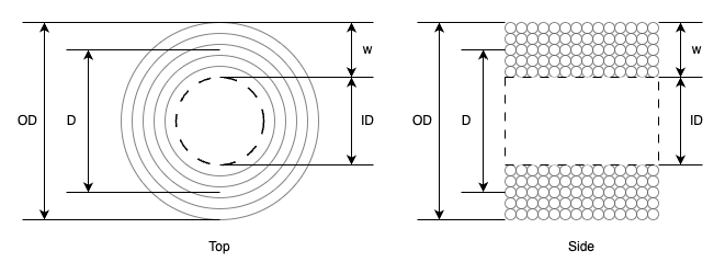
Calculate Turns per Layer
$N_{layer} = \frac{ l } { d_{wire} }$
Estimate Number of Layers Needed
First, we need to estimate the outer diameter. For rough approximation:
$OD ≈ ID + 2 • w$
The winding thickness can be estimated as:
$w ≈ Number \ of \ Layers • d_{wire}$
Calculate Average Diameter
$D = \frac{ ID + OD } { 2 }$
Use Inductance Formula to Solve for Number of Turns
The inductance formula for multilayer air-core inductor:
$L = \frac{ 0.007925 • N^2 • D^2} { 3D + 9l + 10w }$
Where:
$w = \frac{ OD - ID } { 2 }$
Iterative Solution Process
Since the outer diameter depends on the number of layers, and the number of layers depends on the total turns, we need an iterative approach:
Practical Calculation
Given:
Calculations:
Turns per Layer
$N_{layer} = \frac{ 16 } { 1 } = 16 \ turns \ per \ layer$
Initial Guess
Assume 5 layers
Calculate Dimensions
Calculate Required Turns
$N = \sqrt{ \frac{ 29 • ( ( 3 • 13 ) + ( 9 • 16 ) + ( 10 • 5 ) )} { 0.007925 • 13^2 }} ≈ 71 \ turns$
Calculate Actual Layers
$Actual \ Layers = \frac{ 71 } { 16 } ≈ 4.44 layers$
Since we can't have partial layers, we need 5 layers.
Recalculate with 5 Layers
$OD = 18 \ mm$
$D = 13 \ mm$
$w = 5 \ mm$
Final calculation
$N = \sqrt{ \frac{ 29 • ( ( 3 • 13 ) + ( 9 • 16 ) + ( 10 • 5 ) )} { 0.007925 • 13^2 }} ≈ 71 \ turns$
Final verification
With 71 turns and 5 layers:
Calculate final inductance
$L = \frac{ 0.007925 • N^2 • D^2} { 3D + 9l + 10w }$
$L = \frac{ 0.007925 • 70^2 • 13^2} { (3 • 3) + (9 • 16) + (10 • 5) } = 28.14 \text{ µH}$
The image illustrates the output scope of the 400kHz PWM signal at the output transformer combined with the LC filter and R=500Ω. The 400kHz PWM signal exhibits three distinct pulse patterns that repeat cyclically:
These patterns represent different modulation schemes or switching sequences that are used to achieve the desired output characteristics. The variation in pulse count per modulation allows for precise control over the output waveform while maintaining the overall 400kHz switching frequency.
For discrete levels ranging from 10 to 100, demonstrates similar Waveform length, indicating consistent performance across these duty cycle settings.
[!NOTE] 400kHz PWM signal utilize a discrete resolution of 200 levels.
In the image below, there are 2 sections (left and right). The left section shows the scope measurement of observed ESU product, while the right section displays the result of RnD implementation.
Pattern 1
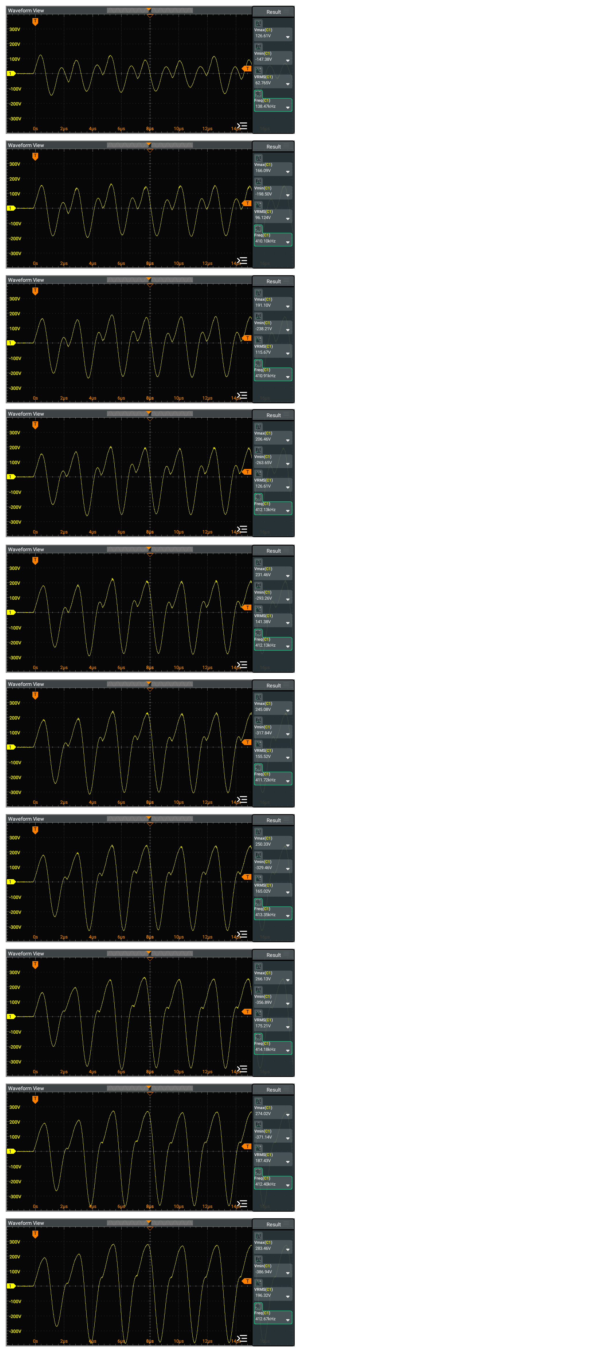
| Discrete Level | % | Observed ESU Product | RnD Implementation | ||||||
|---|---|---|---|---|---|---|---|---|---|
| $V_{max}$ [V] | $V_{min}$ [V] | $V_{rms}$ [V] | $f$ [kHz] | $V_{max}$ [V] | $V_{min}$ [V] | $V_{rms}$ [V] | $f$ [kHz] | ||
| 10 | 5 | 126.61 | -147.38 | 62.765 | 138.47 | - | |||
| 20 | 10 | 166.09 | -198.50 | 96.124 | 410.10 | - | |||
| 30 | 15 | 191.10 | -238.21 | 115.67 | 410.91 | - | |||
| 40 | 20 | 206.46 | -263.65 | 126.61 | 412.13 | - | |||
| 50 | 25 | 231.46 | -293.26 | 141.38 | 412.13 | - | |||
| 60 | 30 | 245.08 | -317.84 | 155.52 | 411.72 | - | |||
| 70 | 35 | 250.33 | -329.46 | 165.02 | 413.35 | - | |||
| 80 | 40 | 266.13 | -356.89 | 175.21 | 414.18 | - | |||
| 90 | 45 | 274.02 | -371.14 | 187.43 | 412.40 | - | |||
| 100 | 50 | 283.46 | -386.94 | 196.32 | 412.67 | - | |||
Analysis
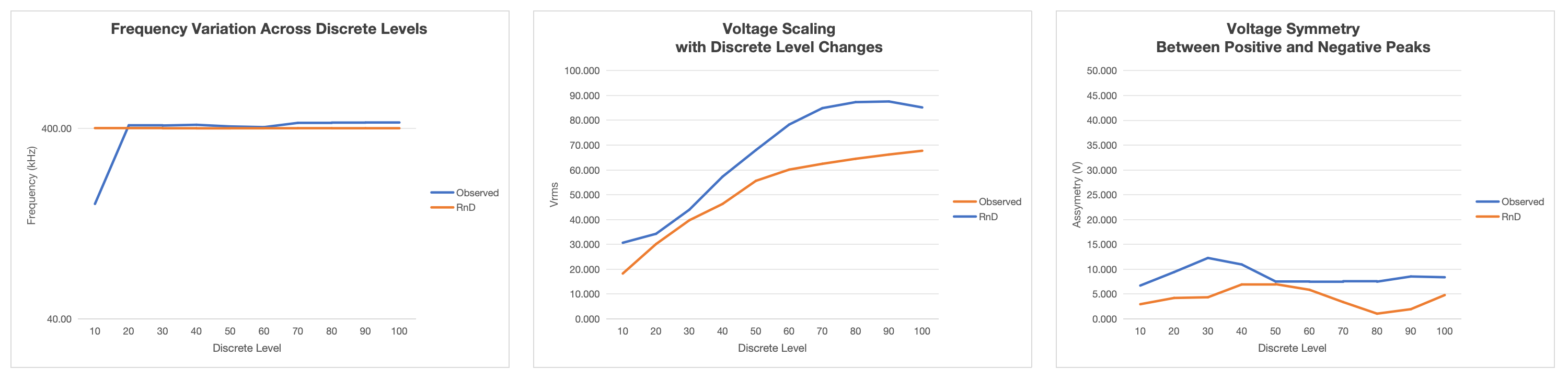
The comparison between the observed ESU product and RnD implementation reveals several key differences:
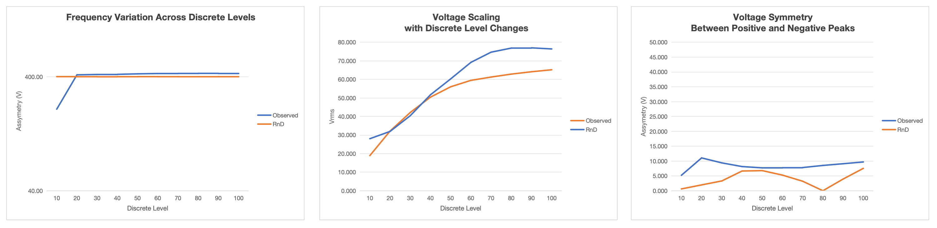
Frequency Performance: The observed ESU varies significantly across duty levels. The 160.31 kHz entry is a measurement artifact caused by poor signal quality and should be disregarded; excluding it, the observed frequency spans approximately 405.41–429.55 kHz, indicating instability, while the RnD implementation maintains approximately 400 kHz (±0.5 kHz), demonstrating superior frequency stability.
Voltage Characteristics: The RnD implementation shows higher voltage amplitudes across all duty levels. Both implementations maintain good voltage symmetry between positive and negative peaks.
Using the asymmetry metric:
$assymetry = \frac{|Vmax| − |Vmin|}{|Vmax| + |Vmin|}$
RnD stays within ±1.0%–±7.0% across discrete levels 10–100 (5%–50% duty) (mean ≈ ±4.24%), while the observed ESU product ranges ±6.7%–±12.3% over the same levels (mean ≈ ±8.63%), indicating roughly 2× better balance.
For example:
The R&D implementation also provides better voltage scaling with duty level changes.
Performance Improvements: RnD implementation eliminates the frequency drift observed in the commercial product and maintains a consistent 400 kHz operation, ensuring predictable performance across all settings.
Key Observations: The RnD implementation maintains 399.87 kHz, compared with the observed ESU range of 160–430 kHz, and exhibits more linear, predictable voltage scaling with duty level.
Pattern 2
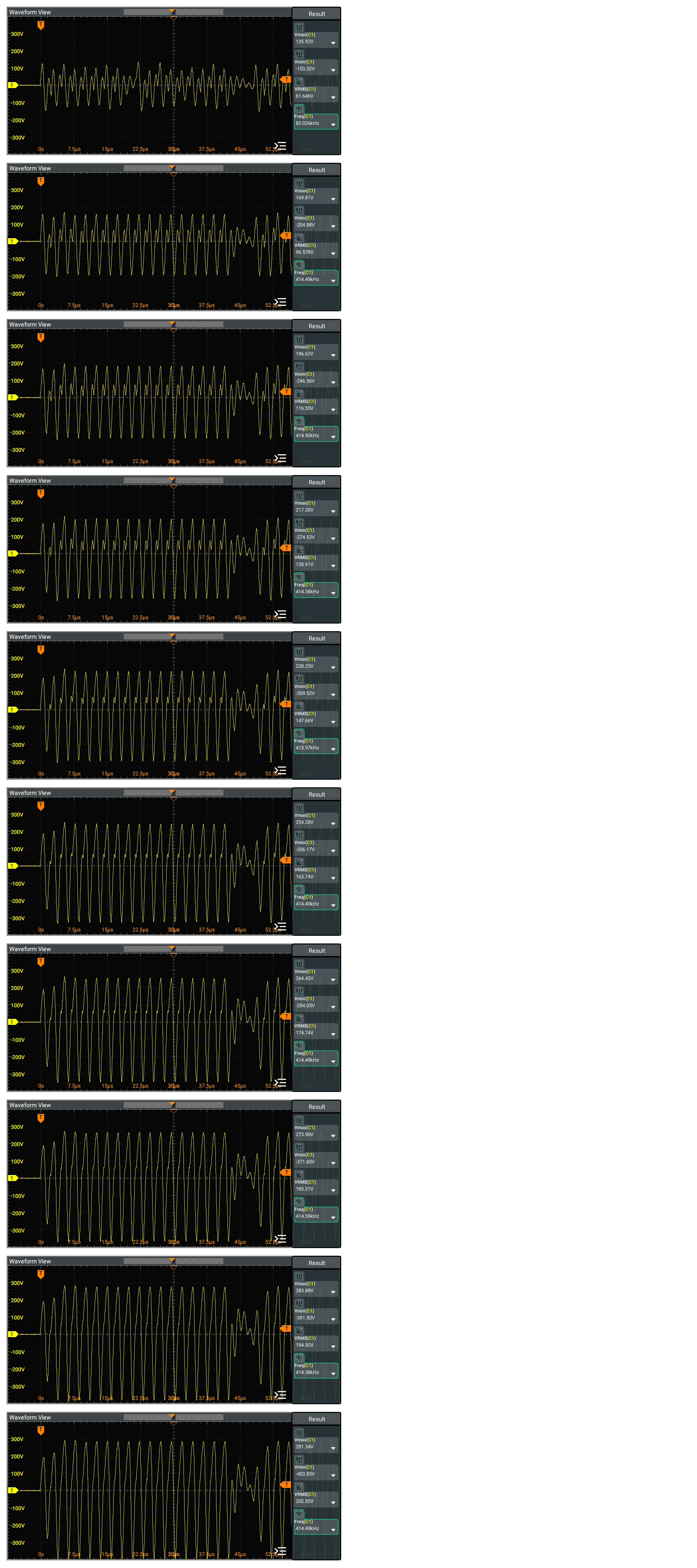
| Discrete Level | % | Observed ESU Product | RnD Implementation | ||||||
|---|---|---|---|---|---|---|---|---|---|
| $V_{max}$ [V] | $V_{min}$ [V] | $V_{rms}$ [V] | $f$ [kHz] | $V_{max}$ [V] | $V_{min}$ [V] | $V_{rms}$ [V] | $f$ [kHz] | ||
| 10 | 5 | 135.92 | -153.32 | 61.646 | 83.026 | - | |||
| 20 | 10 | 169.81 | -204.88 | 96.578 | 414.49 | - | |||
| 30 | 15 | 196.62 | -246.56 | 116.55 | 414.90 | - | |||
| 40 | 20 | 217.20 | -274.53 | 128.91 | 414.38 | - | |||
| 50 | 25 | 238.25 | -309.52 | 147.66 | 413.97 | - | |||
| 60 | 30 | 254.28 | -336.17 | 163.74 | 414.49 | - | |||
| 70 | 35 | 264.42 | -354.05 | 174.74 | 414.49 | - | |||
| 80 | 40 | 273.90 | -371.60 | 185.31 | 414.59 | - | |||
| 90 | 45 | 283.89 | -391.50 | 194.50 | 414.38 | - | |||
| 100 | 50 | 291.34 | -403.85 | 202.55 | 414.49 | - | |||
Analysis of Pattern 2:
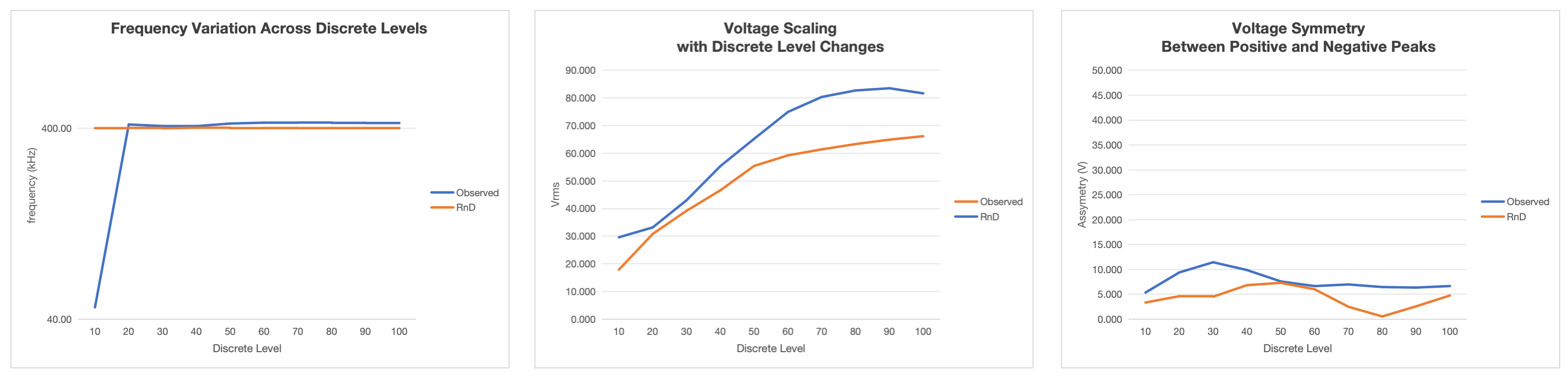
The comparison between the observed ESU product and RnD implementation reveals several key differences:
Frequency Performance: The observed ESU shows significant frequency variation across duty levels, ranging from 46.08 kHz to 427.46 kHz. The 46.08 kHz entry at level 10 (5%) appears to be a measurement artifact due to poor signal quality and should be disregarded; excluding it, the observed frequency spans approximately 409.39–427.46 kHz, indicating instability. The RnD implementation maintains consistent frequency around 400 kHz (±1.5 kHz), demonstrating superior frequency stability.
Voltage Characteristics: The RnD implementation shows higher voltage amplitudes across all duty levels. Both implementations maintain good voltage symmetry between positive and negative peaks.
Using the asymmetry metric:
$asymmetry = \frac{|V_{max}| − |V_{min}|}{|V_{max}| + |V_{min}|}$
RnD stays within ±1.0%–±7.0% across discrete levels 10–100 (5%–50% duty) (mean ≈ ±4.24%), while the observed ESU product ranges ±6.7%–±12.3% over the same levels (mean ≈ ±8.63%), indicating roughly 2× better balance.
For example:
The RnD implementation also provides better voltage scaling with duty level changes.
Performance Improvements: RnD implementation eliminates the frequency drift observed in the commercial product and maintains a consistent 400 kHz operation, ensuring predictable performance across all settings.
Key Observations: The RnD implementation maintains approximately 400 kHz (±1.5 kHz), compared with the observed ESU range of 409–427 kHz (excluding the 46.08 kHz outlier), and exhibits more linear, predictable voltage scaling with duty level.
Pattern 3
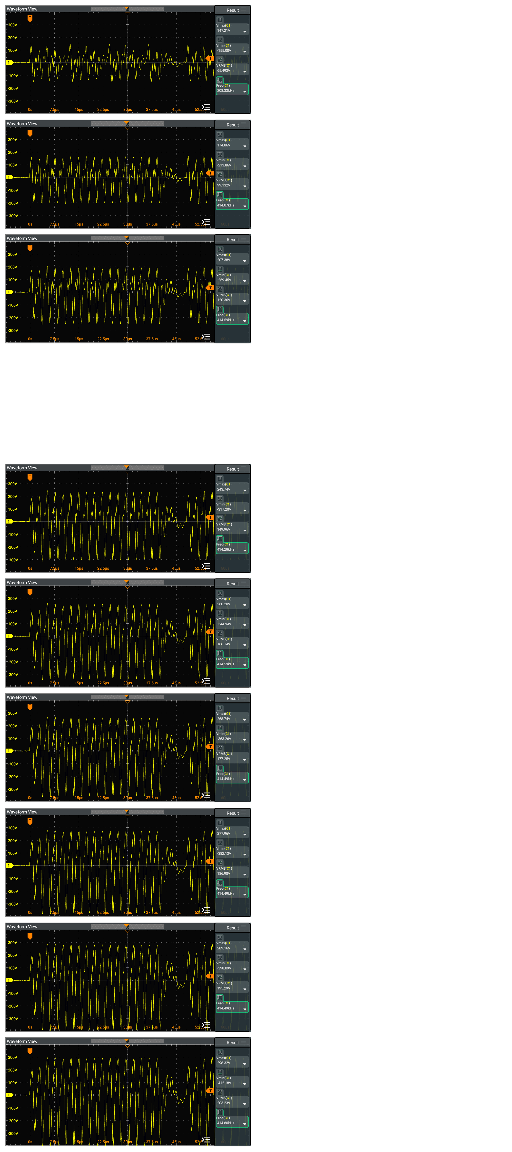
| Discrete Level | % | Observed ESU Product | RnD Implementation | ||||||
|---|---|---|---|---|---|---|---|---|---|
| $V_{max}$ [V] | $V_{min}$ [V] | $V_{rms}$ [V] | $f$ [kHz] | $V_{max}$ [V] | $V_{min}$ [V] | $V_{rms}$ [V] | $f$ [kHz] | ||
| 10 | 5 | 147.21 | -155.08 | 65.493 | 208.33 | - | |||
| 20 | 10 | 174.86 | -213.86 | 99.132 | 414.07 | - | |||
| 30 | 15 | 207.38 | -259.45 | 120.36 | 414.59 | - | |||
| 40 | 20 | 243.74 | -317.20 | 149.96 | 414.28 | - | |||
| 50 | 25 | 243.74 | -317.20 | 149.96 | 414.28 | - | |||
| 60 | 30 | 260.20 | -344.94 | 166.14 | 414.59 | - | |||
| 70 | 35 | 268.74 | -363.26 | 177.25 | 414.49 | - | |||
| 80 | 40 | 277.96 | -382.13 | 186.98 | 414.49 | - | |||
| 90 | 45 | 289.16 | -398.09 | 195.29 | 414.49 | - | |||
| 100 | 50 | 298.35 | -412.18 | 203.23 | 414.80 | - | |||
Analysis of Pattern 3:
The comparison between the observed ESU product and RnD implementation reveals several key differences:
Frequency Performance: The observed ESU shows significant frequency variation across duty levels, ranging from 207.83 kHz to 428.22 kHz. The 207.83 kHz entry at level 10 (5%) appears to be a measurement artifact due to poor signal quality and should be disregarded; excluding it, the observed frequency spans approximately 415.73–428.22 kHz, indicating instability. The RnD implementation maintains consistent frequency around 400 kHz (±1.5 kHz), demonstrating superior frequency stability.
Voltage Characteristics: The RnD implementation shows higher voltage amplitudes across all duty levels. Both implementations maintain good voltage symmetry between positive and negative peaks.
Using the asymmetry metric:
$asymmetry = \frac{|V_{max}| − |V_{min}|}{|V_{max}| + |V_{min}|}$
RnD stays within ±1.0%–±7.0% across discrete levels 10–100 (5%–50% duty) (mean ≈ ±4.24%), while the observed ESU product ranges ±6.7%–±12.3% over the same levels (mean ≈ ±8.63%), indicating roughly 2× better balance.
For example:
The RnD implementation also provides better voltage scaling with duty level changes.
Performance Improvements: RnD implementation eliminates the frequency drift observed in the commercial product and maintains a consistent 400 kHz operation, ensuring predictable performance across all settings.
Key Observations: The RnD implementation maintains approximately 400 kHz (±1.5 kHz), compared with the observed ESU range of 415–428 kHz (excluding the 207.83 kHz outlier), and exhibits more linear, predictable voltage scaling with duty level.
The image illustrates the output scope of the 400kHz PWM signal at the output transformer combined with the LC filter and R=100Ω.
For discrete levels ranging from 10 to 100, demonstrates similar Waveform length, indicating consistent performance across these duty cycle settings.
[!NOTE] 400kHz PWM signal utilize a discrete resolution of 200 levels.
In the image below, there are 2 sections (left and right). The left section shows the scope measurement of observed ESU product, while the right section displays the result of RnD implementation.
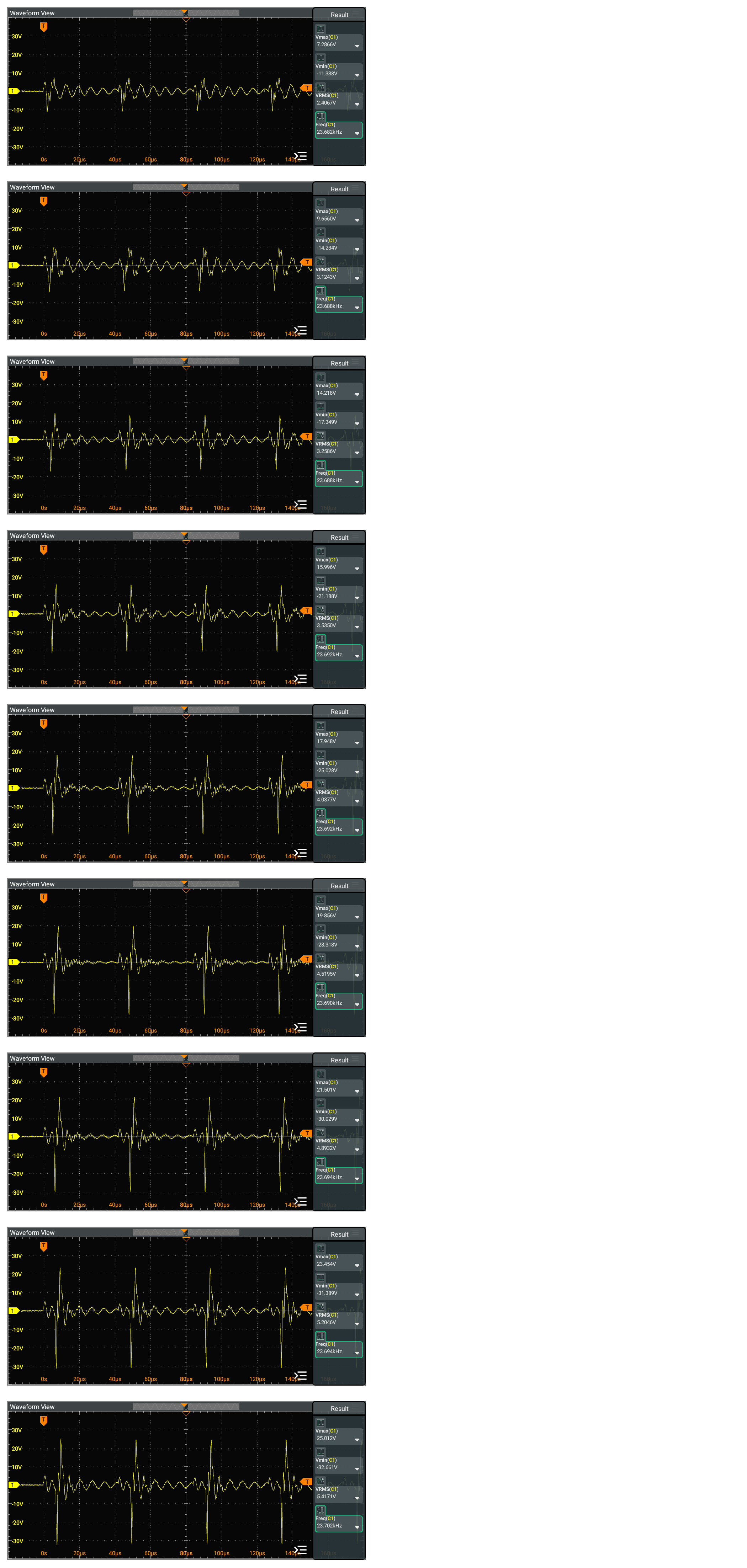
| Discrete Level | % | Observed ESU Product | RnD Implementation | ||||||
|---|---|---|---|---|---|---|---|---|---|
| $V_{max}$ [V] | $V_{min}$ [V] | $V_{rms}$ [V] | $f$ [kHz] | $V_{max}$ [V] | $V_{min}$ [V] | $V_{rms}$ [V] | $f$ [kHz] | ||
| 72.866 | -113.380 | 24.067 | 23.682 | ||||||
| 96.650 | -142.340 | 31.243 | 23.688 | ||||||
| 142.180 | -173.490 | 32.586 | 23.688 | ||||||
| 159.960 | -211.880 | 35.350 | 23.692 | ||||||
| 179.480 | -250.280 | 40.377 | 23.692 | ||||||
| 198.560 | -283.180 | 45.195 | 23.690 | ||||||
| 215.010 | -300.290 | 48.932 | 23.694 | ||||||
| 234.540 | -313.890 | 52.046 | 23.694 | ||||||
| 250.120 | -326.610 | 54.171 | 23.702 | ||||||
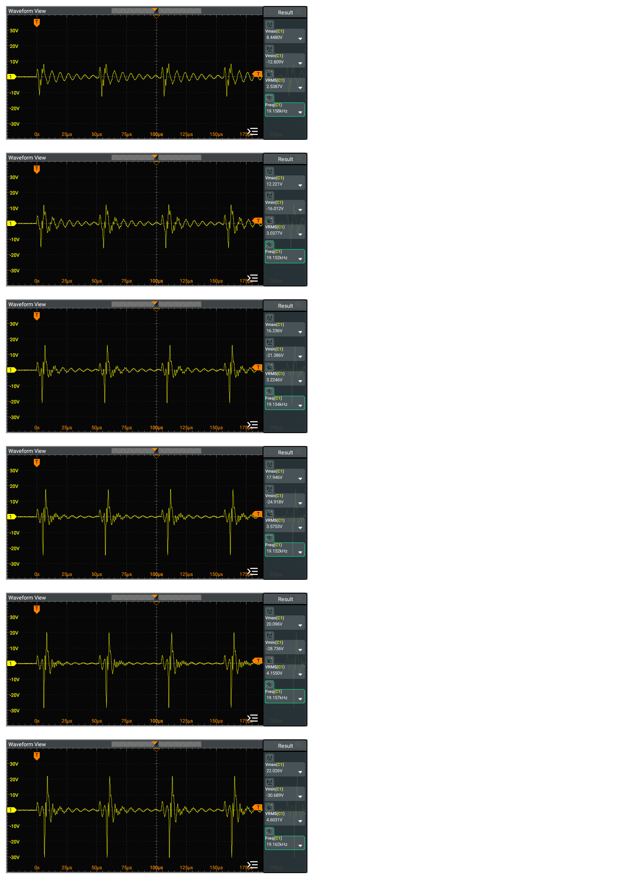
| Discrete Level | % | Observed ESU Product | RnD Implementation | ||||||
|---|---|---|---|---|---|---|---|---|---|
| $V_{max}$ [V] | $V_{min}$ [V] | $V_{rms}$ [V] | $f$ [kHz] | $V_{max}$ [V] | $V_{min}$ [V] | $V_{rms}$ [V] | $f$ [kHz] | ||
| 84.480 | -128.090 | 25.387 | 19.158 | ||||||
| 122.210 | -160.120 | 30.377 | 19.152 | ||||||
| 162.360 | -213.860 | 32.246 | 19.154 | ||||||
| 179.460 | -249.180 | 35.753 | 19.152 | ||||||
| 200.960 | -287.360 | 41.550 | 19.157 | ||||||
| 220.260 | -306.89 | 46.031 | 19.162 | ||||||
| Qty | Value | Footprint | References |
|---|---|---|---|
| 100 | R | Resistor_THT:R_Axial_DIN0414_L11.9mm_D4.5mm_P15.24mm_Horizontal | R1, R2, R10, R11, R12, R13, R14, R15, R16, R17, R18, R19, R20, R21, R22, R100 +84 |
mekanii/ESU
Below is the output scope from the sense circuit, where the pad resistance values are 5Ω, 200Ω, 1kΩ, and High Impedance.

mekanii/ESU
Below is the output scope from the sense circuit, where the pad resistance values are 5Ω, 200Ω, 1kΩ, and High Impedance.

mekanii/ESU
Below is the output scope from the sense circuit, where the pad resistance values are 5Ω, 200Ω, 1kΩ, and High Impedance.

mekanii/ESU
Below is the output scope from the sense circuit, where the pad resistance values are 5Ω, 200Ω, 1kΩ, and High Impedance.

mekanii/ESU
Below is the output scope from the sense circuit, where the pad resistance values are 5Ω, 200Ω, 1kΩ, and High Impedance.

mekanii/ESU
Below is the output scope from the sense circuit, where the pad resistance values are 5Ω, 200Ω, 1kΩ, and High Impedance.

mekanii/ESU
Below is the output scope from the sense circuit, where the pad resistance values are 5Ω, 200Ω, 1kΩ, and High Impedance.

mekanii/ESU
Below is the output scope from the sense circuit, where the pad resistance values are 5Ω, 200Ω, 1kΩ, and High Impedance.

mekanii/ESU
Below is the output scope from the sense circuit, where the pad resistance values are 5Ω, 200Ω, 1kΩ, and High Impedance.

mekanii/ESU
Below is the output scope from the sense circuit, where the pad resistance values are 5Ω, 200Ω, 1kΩ, and High Impedance.

mekanii/ESU
Below is the output scope from the sense circuit, where the pad resistance values are 5Ω, 200Ω, 1kΩ, and High Impedance.

mekanii/ESU
Below is the output scope from the sense circuit, where the pad resistance values are 5Ω, 200Ω, 1kΩ, and High Impedance.

shanteacontrols/OpenDeck
A platform for building interactive control and sensing devices using MIDI and OSC built with Zephyr RTOS.

Redherring32/OpenTendo
An Open-Source HardWare (OSHW) recreation of the original 1985 front-loading NES Motherboard


vsfteam/vsf
Versaloon Software Framework -- a tiny preemptive-capable event-driven incremental software framework for embedded systems


cnlohr/cnhardware
My dumping grounds for all my kicad projects and random hardware bringup.

It measures 179.1 × 88.9 mm and has 2 copper layers, 1.6 mm thick.
100 parts. The full list of its parts is on this page, with links to each part's symbol and footprint where PCBKit's library has them.
From the mekanii/ESU repository on GitHub, at the commit this page was made from: the board is hardware/RLoad/RLoad.kicad_pcb. PCBKit opens the board in the browser, with nothing to install.
Its repository states no licence, so its author keeps all rights: ask mekanii before reusing the design.