
2 layers84 × 85 mm
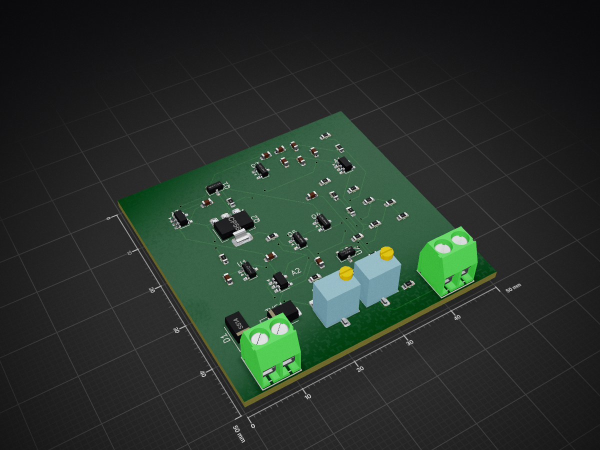
Fully analog 2-wire 4-20 mA NTC thermistor temperature transmitter, built from multi-sourced parts — plus an instrumentation-theory tutorial. Default build: 20-40 C for chocolate temperature control.
Therm is an open-source printed circuit board by ControlSystemIntegrators, from the ControlSystemIntegrators/Therm_temp_4_20_xmtr repository on GitHub, published under the MIT licence. It is a 4-layer board of 50 × 50 mm with 45 parts on 24 nets, routed with 171 tracks and 47 vias.
It is built around the MMBT3904, MMBT3906 and BCP56, with the SMAJ33A and SS14 among its other parts. Its parts include 18 resistors, 11 capacitors, 5 transistors, 2 ICs and 2 connectors.


A fully analog (no microcontroller) 2-wire 4–20 mA temperature transmitter built from standard, multi-sourced parts — and a worked tutorial in the instrumentation theory behind it.
It does two jobs:
Why analog? You can absolutely bolt a microcontroller and a 12-bit ADC on top of this for fine digital adjustment — see Optional digital upgrade. In practice, for "hold a setpoint in a known band" process control, that layer is rarely worth the complexity. This project deliberately stays in the analog domain so the whole signal path is visible and every part is replaceable.
Not a safety device. This is a process measurement instrument, not a safety-rated (SIL) one. Don't use it as a protective function.
| Parameter | Value |
|---|---|
| Output | 4–20 mA, 2-wire loop-powered |
| Loop supply | 7–30 V (24 V typical) |
| Default range | 20–40 °C → 4–20 mA (chocolate) |
| Sensor | NTC thermistor, 10 kΩ @ 25 °C, β ≈ 3892 K (e.g. Omega 44006) |
| In-band accuracy | ±0.1 °C over the 20 °C band (realistic system figure; the electronics + linearization contribute only ~±0.06 °C — sensor interchangeability, self-heating and lead effects dominate) |
| Calibration | zero + span trimpots, non-interactive |
| Quiescent current | ~2.6 mA (fits under the 4 mA floor) |
| Components | jellybean / multi-sourced; op-amps in SOT-23-5 |
Outside the chosen band the output saturates near 4 mA (cold) or 20 mA (hot) — intentional. Accuracy is only specified inside the band.
The current loop. A 2-wire transmitter sits in series with a DC supply and a receiver. The transmitter's job is to draw a controlled current from the loop — 4 mA represents the bottom of the range, 20 mA the top — regardless of loop voltage or wiring resistance (within limits). Because the current is the signal, voltage drops in long cable runs don't corrupt the reading, and a broken wire reads 0 mA (a detectable fault, distinct from a valid 4 mA "low"). That noise immunity and fault detection is why 4–20 mA has survived for decades in industry.
Loop-powered ("2-wire"). The same two wires that carry the signal also power the transmitter. The catch: the entire circuit must run on less than 4 mA, because that floor is the lowest the loop ever provides. Every microamp the electronics draw is part of the loop current, so the design budgets quiescent current carefully and lets an output ("dump") transistor make up the difference to hit the commanded 4–20 mA.
Why a thermistor? An NTC thermistor is cheap, has a large signal (thousands of ohms change over our band), is available with tight interchangeability (±0.1–0.2 °C for the Omega 44000 series), and needs no cold-junction compensation like a thermocouple. Its one drawback is that it is very nonlinear — which is the interesting part of this design.
An NTC's resistance is approximately
R(T) = R25 · exp( β · (1/T − 1/298.15) ) [T in kelvin]For our 10 kΩ part that's ~57 kΩ at −10 °C falling to ~3.6 kΩ at +50 °C — about 15:1, and badly curved. Fed straight into a linear amplifier you'd get large errors away from one calibration point.
The fix is a single resistor in parallel with the thermistor. The parallel
combination Rt ∥ Rlin has an S-shaped curve with an inflection point; placing
that inflection at the center of your band makes the network resistance very
nearly linear in temperature there. The value for maximum linearity at center
temperature Tc (kelvin) is:
Rlin = Rt(Tc) · (β − 2·Tc) / (β + 2·Tc)For the chocolate build (center 30 °C) the closed-form (unloaded) value is ~5.9 kΩ; the build uses 6.04 kΩ, re-optimized for the gain-stage loading (see below). Either way the residual nonlinearity across 20–40 °C is only ~±0.06 °C — comfortably inside the ±0.1 °C system spec, so the linearization is never the limiting term.
A second resistor can add a curvature-shaping term (by exciting through a divider instead of a constant current), so we checked whether it's worth it. For an NTC it essentially isn't — the optimizer drives the second resistor back toward "constant current," and the conformity barely moves:
| Band → 4–20 mA | 1 resistor | 2 resistors |
|---|---|---|
| 20–40 °C | ±0.061 °C | ±0.057 °C |
| 15–45 °C | ±0.207 °C | ±0.188 °C |
| −10–50 °C | ±1.585 °C | ±1.545 °C |
~5% improvement for an extra precision part and an extra calibration interaction. We dropped it. The real lever is band width, not resistor count (see the table — the wider the band, the worse the conformity). Pick the narrowest band that covers where your process actually operates.
There's a subtle trap the ideal math hides. The single-op-amp difference amp
(next stage) presents its input network — R9 + R12 from the sensor node to
ground — as a load on node X. The sensor's source impedance there is the
linearized network (a few kΩ), so a low input impedance bleeds a
temperature-dependent current out of the node and bows V(X), adding
nonlinearity the zero/span trims cannot remove.
We only caught this with the device-level SPICE model (the ideal netlist and
the first cut of design.py both assumed an infinite-impedance gain input). With
the original 10 k / 24.9 k divider (R9+R12 ≈ 35 kΩ) loading a ~4 kΩ source, the
in-band conformity blew out to ±0.18 °C — past the spec. Two fixes, both
verified:
R9=R10=100 kΩ, R11=R12=249 kΩ (R9+R12 ≈ 349 kΩ, ~1 % loading).design.py now models the
load (--rload) and searches for the best linearization resistor rather than
trusting the unloaded closed form (hence 6.04 kΩ, not 5.9 kΩ).With both, conformity is back to ±0.058 °C, confirmed in the device-level sim. Lesson: a difference amp driven from a non-trivial source impedance must have an input impedance well above it, or you pay for it in linearity.
You can reproduce all of this — and design for your own sensor/range — with
tools/design.py.
Two views: the signal chain (what computes the current) and the power/output loop (how a 2-wire device powers itself and sets loop current).
 Vref(2.5V) ──[ NTC ∥ Rlin ]──● X ─────────────►┌────────────┐
                              │                 │   A2       │
              A1 sinks Iexc ──┘                 │ gain/zero  │─ Vcmd ─►┌──────────┐
              (0.25 mA, constant)               │  (2 pots)  │         │ A3 servo │─► loop
                                                └────────────┘         │  + Q2    │   current
   V(X) = Vref − Iexc·(NTC ∥ Rlin)                                     └──────────┘
        (rises with temperature)        Vcmd = SPAN·(V(X) − ZERO)   Iloop = Vcmd / Rsense
A constant current is pulled through the linearized network, so the node voltage
V(X) is a clean, near-linear function of temperature. The gain/zero amplifier
scales and offsets it; the output stage turns that command voltage into loop
current.
 LOOP+ ──▷|──┬───────────────────────────────┬──────────► IN (raw 7..30 V)
   (24 V) D1 │                               │
           TVS         pre-reg: Q1 + TL431 ───┤────────► VL (+5 V) ─► Vref, A1, A2, A3
            │          (series NPN follower)  │
            │                                 └────────► Q2 collector (dump)
            │                                                  │ emitter
 LOOP- ─────┴────────────────[ Rsense 50Ω ]──────  AGND ───────┘
                                    ▲
                A3 drives Q2 so that  Iloop · Rsense = Vcmd
Everything returns to AGND and flows out through Rsense, so the
sense resistor sees the total loop current — the electronics' own ~2.6 mA
quiescent draw plus whatever the dump transistor Q2 adds. A3 servos Q2 until
that total equals Vcmd / Rsense. Because quiescent draw (~2.6 mA) is below the
4 mA floor, Q2 always has something to add.
| Stage | Parts | Function | Key relation |
|---|---|---|---|
| Protection | D1 (Schottky), TVS | reverse-polarity + surge | — |
| Pre-regulator | Q1 (NPN follower), TL431, divider, + Q4/Q5 bias source | makes the +5 V rail VL from the loop; series pass, not shunt, so it draws only what the electronics need. Q4/Q5 form a 2-transistor constant-current source (a jellybean replacement for a current-regulating diode) that biases the TL431 flat across the 7–30 V loop | VL = 2.5·(1+Rfa/Rfb) |
| Reference | LM4040-2.5 | 2.500 V for excitation + zero | — |
| Excitation | A1, Q3, Rexc | constant Iexc = Vref/Rexc = 0.25 mA pulled through NTC∥Rlin | V(X)=Vref − Iexc·Rnet |
| Linearization | Rlin (6.04 kΩ) | straighten the curve in-band | Rlin = Rt(Tc)·(β−2Tc)/(β+2Tc), re-optimized for load |
| Gain/Zero | A2 + span pot + zero pot | scale & offset to the command voltage | Vcmd = SPAN·(V(X) − ZERO) |
| Output | A3, Q2, Rsense | servo loop current to the command | Iloop = Vcmd / Rsense |
The three knobs are orthogonal, which makes calibration sane: Rlin depends only on the band center, span on the band width, and zero on the band position. Move the band up/down → re-zero only. Widen it → re-span only. Re-center it → change Rlin.
Run the calculator with your sensor and the two temperatures you want at 4 mA and 20 mA:
python3 tools/design.py --r25 10000 --beta 3892 --tlow 20 --thigh 40It prints the linearization resistor, the excitation resistor, the span (gain) and zero (offset) targets, the conformity error you'll get, the self-heating estimate, and a transfer table. Defaults are the chocolate build. Output for the default:
--- Linearization ---
Rlin (E96)      : 6.040 kohm   <- re-optimized for gain-stage loading
Conformity      : +/- 0.059 C
--- Excitation ---
Rexc (E96)      : 10.000 kohm  -> Iexc = 0.2500 mA
--- Amplifier / output stage ---
SPAN  (gain)    : 2.5706 V/V   <- set by span pot
ZERO  (Vzero)   : 1.3872 V     <- set by zero pot
Manual recipe (what the script does):
Tc = (Tlow+Thigh)/2; Rlin = Rt(Tc)·(β−2Tc)/(β+2Tc),
rounded to the nearest E96 value.Iexc (~0.25 mA is a good balance of signal size vs.
self-heating); set Rexc = Vref / Iexc.V(X) = Vref − Iexc·(Rt ∥ Rlin) at Tlow and Thigh.SPAN = (20mA−4mA)·Rsense / (V(X)@Thigh − V(X)@Tlow).ZERO so the output is 4 mA at Tlow.Then check the printed conformity. If it exceeds your target, your band is too wide — narrow it (see the table above).
You need a way to present two known temperatures (a stirred ice/water-and-warm
bath, a dry-block calibrator, or — easiest for bench bring-up — two precision
resistors substituted for the probe equal to Rt(Tlow) and Rt(Thigh), which
the calculator prints).
Tlow, e.g. 20 °C → Rt = 12.49 kΩ). Adjust the
ZERO pot for 4.00 mA.Thigh, e.g. 40 °C → Rt = 5.35 kΩ). Adjust the
SPAN pot for 20.00 mA.Use a loop calibrator or a 250 Ω precision resistor + DMM (1.000–5.000 V = 4–20 mA) to read the current.
Every active part below is available from multiple manufacturers, or in a footprint with many drop-in alternatives. That is a design goal: this instrument should be repairable for decades without a single-source IC.
| Ref | Part | Function | Second-source notes |
|---|---|---|---|
| RT1 | NTC 10 kΩ, β≈3892 (Omega 44006 / equiv.) | sensor | any 10k NTC with known β; re-run calculator for other betas |
| Rlin | 6.04 kΩ, 1%, ≤25 ppm/°C | linearization | passive, universal |
| U1 | LM4040-2.5 (2.500 V) | reference | TI, ADI, Diodes, ON |
| U2 | TL431 (2.5 V shunt ref) | pre-reg reference | TI, ON, Diodes, ST, UTC — the multi-sourced jellybean; KiCad sym TL431DBZ (SOT-23) |
| Q1 | NPN small-signal (MMBT3904 / BC847) | pre-reg pass (follower) | universal |
| Q2 | NPN, ~0.5 W (SOT-223, e.g. BCP56 / PZTA42) | output dump transistor | universal; see thermal note |
| Q3 | NPN small-signal (MMBT3904 / BC847) | excitation current sink | universal |
| A1–A3 | µpower precision op-amp, SOT-23-5 (OPA333 / MCP6V31 / TLV9061-class) | excitation, gain/zero, output servo | by exact PN limited; by SOT-23-5 footprint, dozens of swappable parts |
| Rexc | 10.0 kΩ, 1%, ≤25 ppm/°C | sets Iexc | passive |
| Rsense | 49.9 Ω (or 50 Ω), 1%, ≤25 ppm/°C | loop sense | passive |
| Rfa/Rfb | 10.0 kΩ / 10.0 kΩ, 1% | sets VL = 2.5·(1+Rfa/Rfb) = 5 V | passive |
| RV1 | zero trim, SMD multiturn cermet (e.g. 3269 / 3224) | ZERO | universal |
| RV2 | span trim, SMD multiturn cermet | SPAN | universal |
| D1 | Schottky SMA (SS14 / BAT54) | reverse polarity | universal |
| TVS1 | SMAJ33A (or per supply) | surge | universal |
| C1–Cn | 100 nF + 1–10 µF bypass | decoupling | universal |
Thermal note (Q2). A 2-wire transmitter must drop the loop voltage somewhere; that's Q2. Worst case ≈ (instrument voltage) × (loop current) ≈ 20 V × 20 mA ≈ 0.4 W. Use a SOT-223 (or larger) device with adequate copper, or split the drop with a series resistor ahead of Q2's collector.
Op-amp footprint. Standardizing A1–A3 on SOT-23-5 singles is deliberate: precision op-amps are mostly single-source by part number, but the SOT-23-5 single-op-amp pinout is a de-facto industry standard with many footprint- compatible options, so a substitute is always a re-qualification away, never a redesign.
sim/transmitter.cir models the ideal signal chain
(reference + op-amps as behavioral sources, NTC as a temperature-dependent
resistor) and DC-sweeps temperature to confirm the 4–20 mA transfer and in-band
linearity.
ngspice -b sim/transmitter.cir # DC-sweeps temperature; prints Iloop vs T(LTspice: change the behavioral-resistor r='...' syntax to R=....)
It has been run with ngspice 46; the full output is saved in
sim/SIM_RESULTS.txt. Key points (Iloop = Vcmd / 50 Ω):
| T (°C) | V(x) | Vcmd | Iloop |
|---|---|---|---|
| 20 | 1.49812 V | 0.20009 V | 4.00 mA |
| 30 | 1.64825 V | 0.59996 V | 12.00 mA |
| 40 | 1.79854 V | 1.00024 V | 20.00 mA |
| <20 | — | clamps 0.190 V | 3.8 mA (under-range) |
| >40 | — | clamps 1.025 V | 20.5 mA (over-range) |
The node voltages match tools/design.py to the millivolt, and the in-/out-of-
band clamping behaves as designed.
Verification status (be honest about it):
tools/design.py and
confirmed in ngspice (table above).If you later want digital trim, datalogging, or a nonlinear curve over a wide
range, you can add an MCU with a ≥12-bit ADC reading V(X) and driving the loop
via a current-output DAC (or by replacing the A3/Q2 stage). For a "hold a
setpoint in a known band" application this is usually unnecessary complexity —
the analog path here already beats thermocouple accuracy in-band — but the
sensor front-end and linearization theory carry over unchanged.
Taking this from netlist to schematic to PCB surfaced a few KiCad limitations
worth recording — both for anyone reproducing the board and for anyone doing a
careful (or AI-assisted) review of a .kicad_sch:
Connectivity can't be read reliably from the .kicad_sch text. Symbol
mirror/rotation transforms and overlapping wire segments defeat any attempt to
infer "what's connected to what" from pin coordinates. Let KiCad compute it
instead — kicad-cli sch export netlist --format kicadsexpr -o net.net therm.kicad_sch — and read the nets. Every net-by-net review of this board was
done that way, not by eyeballing the schematic file.
ERC does not catch wrong values or wrong roles. Several real errors
here passed connectivity checks clean: a 49.9 kΩ loop-sense resistor that
should have been 49.9 Ω; a bypass cap with both pins on the same net (a
no-op); an op-amp powered from the 2.5 V reference instead of the 5 V rail; and
the LM4040 reference wired across the loop input as if it were the TVS. None of
these trip ERC — they need an explicit value-and-node audit against intent.
Symbol variants have different pin numbering. The OPA333 in SOIC-8
(OPA333xxD) uses pins 2/3/4/6/7; in SOT-23-5 (OPA333xxDBV) it's 1–5. Grab
the wrong variant and the schematic looks right while the netlist is wrong —
always confirm the symbol's package/pinout matches the footprint you intend.
Not every jellybean part is in the stock library. The TL431 is
(Reference_Voltage:TL431DBZ); the TLV431 is not, which had forced a custom
symbol — one reason we standardized on the TL431. Preferring stock-library
parts avoids custom-symbol upkeep.
Footprints aren't auto-assigned. Symbols sit with an empty footprint until you assign one, and nothing warns you until you try to lay out the board — the two trimpots were caught this way. Sweep for missing footprints before routing.
File hygiene. KiCad scatters *-backups/ zips, ~*.lck locks,
#auto_saved_files#, and per-user *.kicad_prl state through the project; the
.gitignore excludes them so only the real design files track.
Takeaway: a parameterized calculator proves the design intent, and ERC proves the nets are connected — but neither flags a wrong value, a wrong package variant, or a node that's electrically valid yet functionally pointless. A net-by-net netlist review plus a device-level SPICE pass are what actually prove the instrument.
Therm_temp_4_20_xmtr/
├── README.md                    # this file
├── LICENSE                      # MIT
├── docs/
│   └── DESIGN_CONVERSATION.md   # the prompts that drove the design + decisions
├── hardware/
│   └── BOM.md                   # bill of materials (consolidated values, tempco notes)
├── tools/
│   └── design.py                # parameterized design calculator (models gain-stage load)
├── sim/
│   ├── transmitter.cir          # ideal transfer-function verification
│   ├── device_level.cir         # discrete model (real BJTs + IC macromodels)
│   └── SIM_RESULTS.txt          # captured ngspice 46 output
└── therm_kicad/                 # KiCad project: schematic + rough PCB
    └── therm/                   # therm.kicad_sch / .kicad_pcb / .kicad_pro
For how this design came to be — the design conversation and the reasoning
behind each choice — see docs/DESIGN_CONVERSATION.md.
Status: schematic + a rough PCB are in therm_kicad/; the device-level SPICE
model verifies the discrete signal chain. Still open: output-stage loop
stability (AC/transient) and bench bring-up.
MIT. Use it, build it, sell it — just keep the copyright notice.
| Qty | Value | Footprint | References |
|---|---|---|---|
| 6 | 100k | PCM_SparkFun-Resistor:R_0603_1608Metric | R5, R9, R10, R13, R14, R18 |
| 6 | 100nF | PCM_SparkFun-Capacitor:C_0603_1608Metric | C1, C5, C7, C9, C10, C11 |
| 3 | 10k | PCM_SparkFun-Resistor:R_0603_1608Metric | R3, R4, R6 |
| 3 | 2.49k | PCM_SparkFun-Resistor:R_0603_1608Metric | R2, R7, R15 |
| 3 | OPA333xxDBV | Package_TO_SOT_SMD:SOT-23-5 | A1, A2, A3 |
| 2 | 1uF | PCM_SparkFun-Capacitor:C_0603_1608Metric | C2, C8 |
| 2 | 249k | PCM_SparkFun-Resistor:R_0603_1608Metric | R11, R12 |
| 2 | 3.5mm | PCM_SparkFun-Connector:ScrewTerminal_1x02_P3.5mm_Horizontal_Black | J1, TB1 |
| 2 | 50k | Potentiometer_SMD:Potentiometer_Bourns_3269W_Vertical | RV1, RV2 |
| 2 | MMBT3904 | Package_TO_SOT_SMD:SOT-23 | Q1, Q3 |
| 2 | MMBT3906 | Package_TO_SOT_SMD:SOT-23 | Q4, Q5 |
| 1 | 100pF | PCM_SparkFun-Capacitor:C_0603_1608Metric | C3 |
| 1 | 10nF | PCM_SparkFun-Capacitor:C_0603_1608Metric | C6 |
| 1 | 1nF | PCM_SparkFun-Capacitor:C_0603_1608Metric | C4 |
| 1 | 2k | PCM_SparkFun-Resistor:R_0603_1608Metric | R8 |
| 1 | 432 | PCM_SparkFun-Resistor:R_0603_1608Metric | R17 |
| 1 | 49.9 | PCM_SparkFun-Resistor:R_0603_1608Metric | R16 |
| 1 | 6.04k | PCM_SparkFun-Resistor:R_0603_1608Metric | R1 |
| 1 | BCP56 | Package_TO_SOT_SMD:SOT-223-3_TabPin2 | Q2 |
| 1 | LM4040DBZ-2.5 | Package_TO_SOT_SMD:SOT-23 | U1 |
| 1 | SMAJ33A | Diode_SMD:D_SMA | TVS1 |
| 1 | SS14 | Diode_SMD:D_SMA | D1 |
| 1 | TL431DBZ | Package_TO_SOT_SMD:SOT-23 | U2 |


EwoudVV/arpeggiator
12-note analog arpeggiator with a 1/2/3 octave range, custom pcb and printed case

danhmanu/PLC-STM32F407VET6
Mạch nguyên lý KiCad 10 cho bộ PLC: điều khiển qua LAN bằng Modbus TCP (module W5500 Lite), nạp code qua USB‑C (CH340C), 16 ngõ ra transistor cách ly quang, 10 ngõ vào analog 4–20mA.


janni0609/2-Channel-PreReg-Powersupply
A two-channel laboratory bench power supply, 0–36 V / 0–2 A per channel, fully isolated between channels. Each channel pairs a tracking switch-mode pre-regulator with a linear post-regulator, so it has the low output…

It measures 50 × 50 mm and has 4 copper layers, 1.6 mm thick.
45 parts, built around the MMBT3904, MMBT3906, BCP56 and SMAJ33A. The full list of its parts is on this page, with links to each part's symbol and footprint where PCBKit's library has them.
From the ControlSystemIntegrators/Therm_temp_4_20_xmtr repository on GitHub, at the commit this page was made from: the board is therm_kicad/therm/therm.kicad_pcb and its schematic therm_kicad/therm/therm.kicad_sch. PCBKit opens the board in the browser, with nothing to install.
Its repository publishes it under the MIT licence: you may reuse it on that licence's terms (keep the author's notice, and for a copyleft licence share your changes alike).