Blog ·
Analyses your agent writes: a circuit and signal simulator in a sandbox
Sergey Alekseev
PCBKit had four lenses: power, current, heat and “is it ready to order”. Each one answers one question and each one answers it well enough but people (and their agents) don’t ask four questions. They ask “are my USB lines 90 Ω”, “will the 3.3 V rail dip when the Wi-Fi transmits”, “is my buck stable”, “why did we fail EMC last time” and every one of those is a different analysis with different numbers going in. Professional tools solve this with a menu of a hundred dialogs. We don’t have a hundred dialogs and honestly I don’t want them.
What we have is an agent that writes code. So an analysis is now a script.
How it works
An analysis script is plain synchronous JavaScript that runs in a sandbox (QuickJS, the same one the device simulator uses for its worlds) on the open board. It has no network, no files and no clock. It has one door out: a host function that takes JSON and calls PCBKit’s solvers, which are Rust (the same code runs natively and as WebAssembly in the page). On the JavaScript side that door looks like a handful of objects:
pcb: the board. Nets, parts, tracks, the stack, a net’s cross-section where it runs, a rail’s power distribution network, where a signal’s return current flows.sim: circuits. DC, AC, transient, noise, DC sweeps, SPICE netlists, IBIS buffers.rf: lines and networks. Field-solved cross-sections, lossy multiconductor lines, Touchstone, S-parameters, TDR, eyes, statistical links, PDN impedance.dsp,thermal,units,math: the rest.out: what the person sees. Findings with a place on the board, curves, heat maps, Smith charts, tables, headline numbers and colours painted over the copper in 2D and 3D.
A script also declares what it asks for: input.number("tolerance", …), input.net("rail", …),
input.current("load", …). Declaring is reading: the call returns the value this run uses. The
page draws these as controls beside the answer (sliders, menus and a little editor for a current
over time: steady, a step, pulses or a sine) and when you move one the script runs again and the
previous answer stays in every chart dashed. That turned out to be the part I like most: you drag
the load current and watch the rail dip deeper.
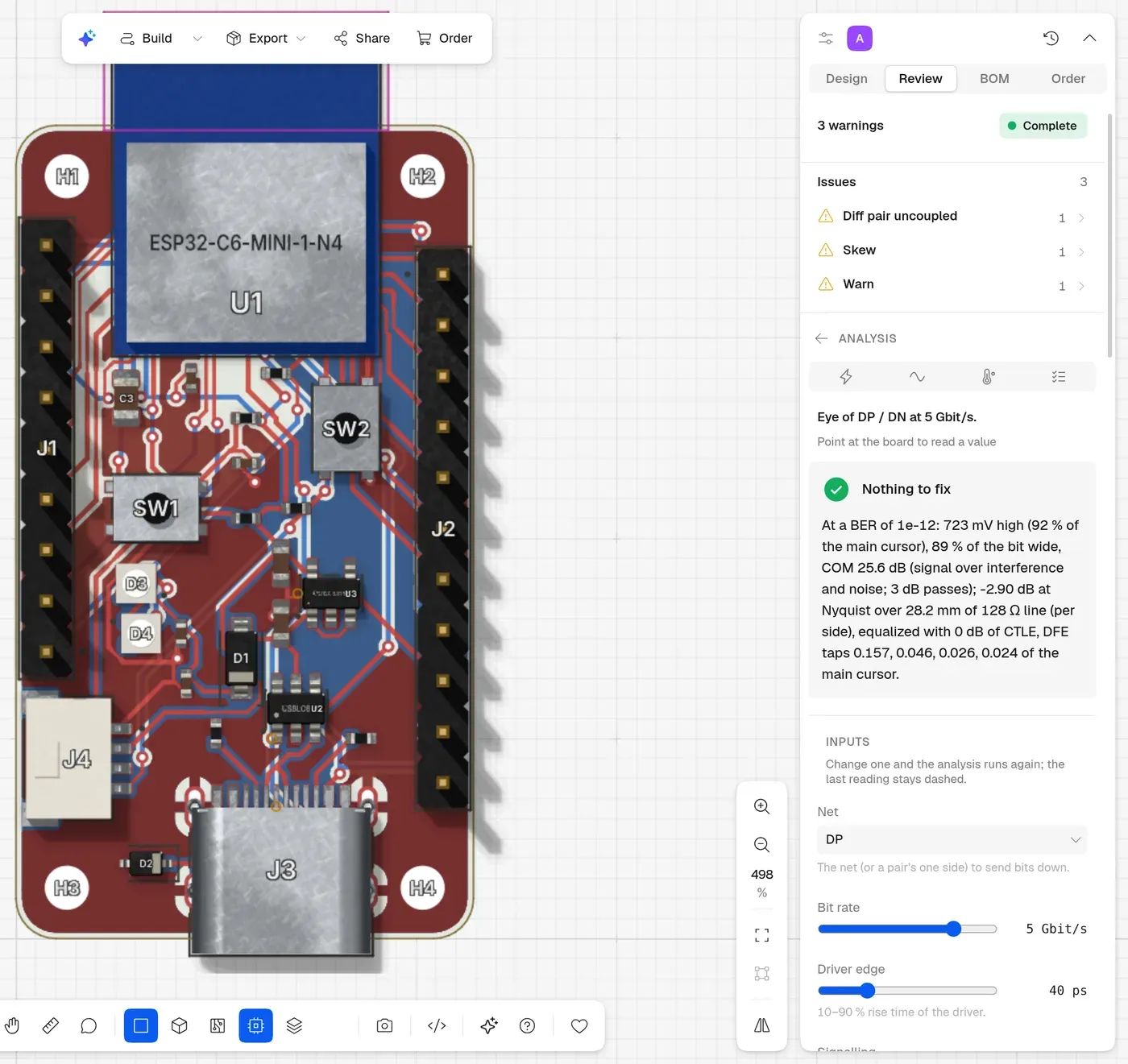
The eye template on an ESP32-C6 board’s USB pair at 5 Gb/s: the answer first, the inputs below it.
There are thirteen templates for the usual questions (impedance, eye, reflections, crosstalk, return paths, emissions, PDN, plane resonances, load steps, switching regulators, heat-up, filter response, tolerances). The agent runs one with the person’s conditions as inputs, or copies one into the board’s repository and changes it, or writes a new one when nothing fits.
What is inside and what we checked it against
A simulator you wrote yourself checked by tests you wrote yourself proves very little, so every solver has an outside reference. ngspice 42 runs on the dev host next to our own build and the decks are the same files.
Circuits. Gummel–Poon transistors, level 1 MOSFETs with the body effect, diodes, junction charge (depletion and diffusion), lossless and lossy transmission lines, controlled and behavioural sources, tables, IBIS buffers. Against ngspice: operating points and DC sweeps within 1 µV, AC within 5·10⁻⁷, noise within 2·10⁻⁷, a diode’s reverse recovery within 0.2 mV, a saturating transistor switch within 10 mV of a 5 V swing, a source follower with its body at ground within 6 µV.
Lossy lines in time. A trace is a lossy line with skin effect and dielectric loss and those are frequency dependent, which a time-domain simulator can’t take directly. So the line becomes sections of exact lossless line with the losses between them as small causal networks: the skin effect as resistor-inductor sections (Kim and Neikirk’s compact model), the dielectric as Debye branches, both fitted by nonnegative least squares. Against the exact line: within 0.2 dB and 3° up to 5 GHz over 20 cm of FR-4. Against ngspice’s LTRA: DC within 10⁻¹³ V and a pulse within 1.5 % on 0.2 ns edges, which is about how much LTRA and a 400-segment RLC ladder in ngspice differ from each other on the same edges.
Impedance. A 2D field solver on the board’s real stack (planes, coplanar grounds, solder mask). Against Hammerstad–Jensen within 0.7 % on FR-4 and 0.01 % in air.
Serial links. The statistical eye that compliance tools compute: every cursor of the pulse response as an independent symbol, their interference convolved exactly, noise and jitter mixed in and the equalization a SerDes would train (transmitter de-emphasis, a CTLE, a DFE) chosen for the best margin. The answer is the eye’s height and width at a bit error ratio, its contours, the bathtub and COM. A PRBS15 run through the same channel gives the same eye height within 2 %.
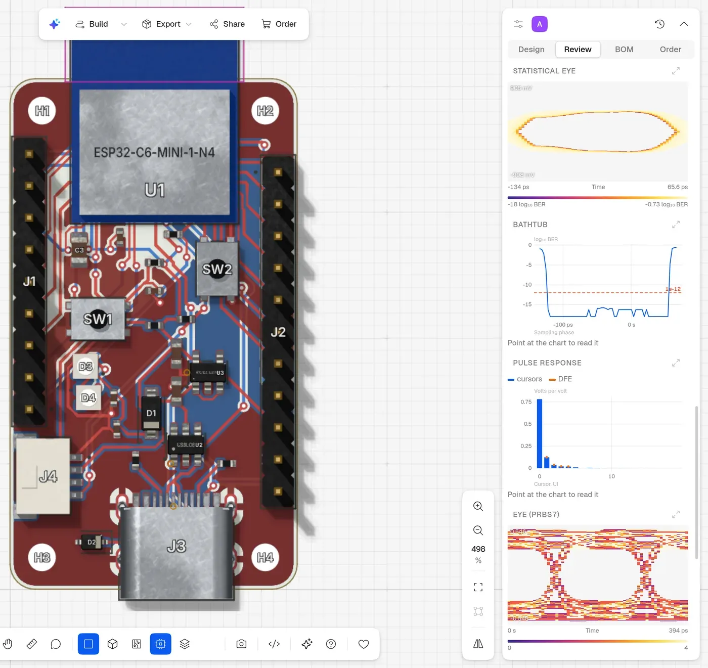
The same pair: the statistical eye (the log of the error ratio over phase and slicer voltage), the bathtub, the cursors and a PRBS7 eye.
Power. A rail’s impedance from its regulator, its capacitors and its planes, with each capacitor’s mounting inductance computed from the layout (the trace to its via, the via pair down to the plane, the planes spreading to the chip), so a capacitor far from the chip helps less just like on the bench. The same network in time for a load step. Plane pairs as a grid of cells for their resonances: a 60 × 40 mm pair rings where c/(2a√εr) says, within 1 %.
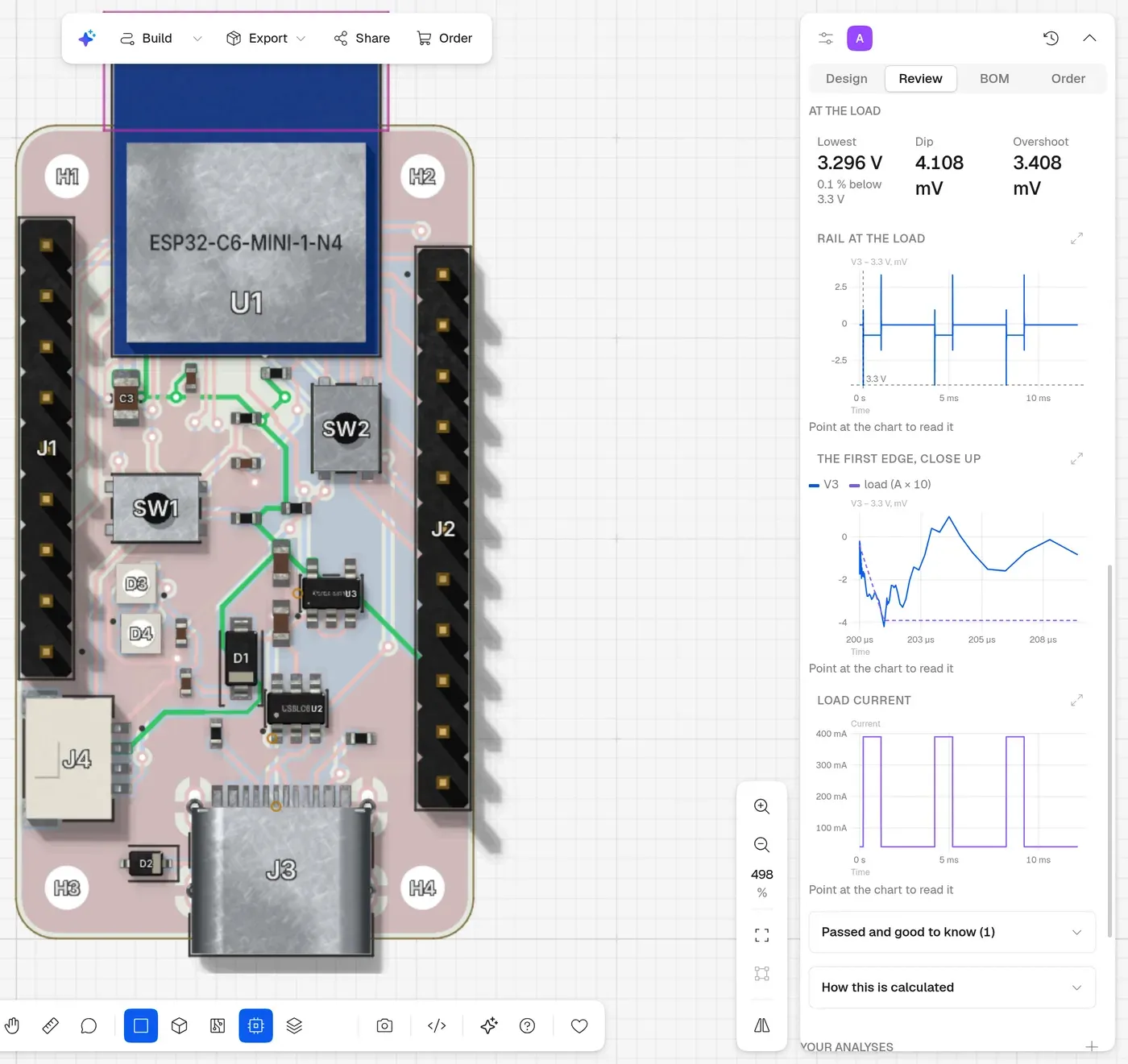
Wi-Fi-like bursts on the 3.3 V rail: 4 mV of dip and the first edge up close.
Switching regulators. The buck’s ripple, peak current against the inductor’s saturation, losses and efficiency and its control loop: voltage mode on an averaged model with type II or type III compensation, or peak current mode with the board’s own COMP network read from the chip’s pin. A loop designed for 30 kHz and 60° lands within 15 % and 8°.
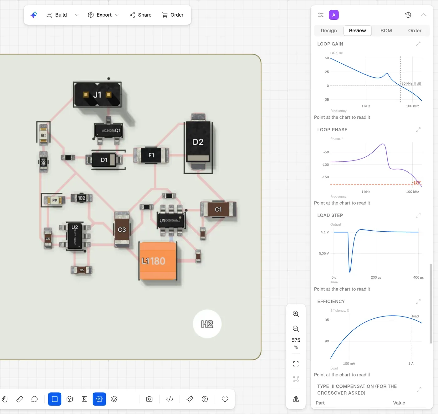
A 12 V to 5 V buck: loop gain and phase, a load step and efficiency over load.
Return paths. Under every track, whatever carries its return current (a pour on the next layer, or a ground pour beside it). A split ground under a track shows up as a gap with its place and the part it’s next to; a layer change without a stitching via or capacitor nearby shows up too.
What broke
Most of the time went into the transient engine, not into the physics.
The trapezoidal rule (what SPICE uses by default) has a well-known habit: where a source’s slope jumps, a capacitor’s current starts ringing step to step and never settles. Our error control compared every device current between a full step and two half steps, so it saw the ringing and kept halving the step until it hit floating point and gave up. It took me embarrassingly long to see that the fix is the one SPICE uses since forever: read the error on the capacitors’ voltages (their charge), not on their currents. Then a large capacitor over a tiny step turned out to be ill-conditioned enough that its own rounding failed the Kirchhoff check, which needed iterative refinement and a backward-error test. And stiff circuits (a chip’s nanosecond die capacitance under millisecond current bursts) needed Gear’s method, because the trapezoidal rule never damps a fast mode, it just rings forever. Each of these was a day of “why is the step 10⁻²⁴ seconds”.
Agents asking real questions
To see if any of this is usable we wrote seven scenarios the way people ask: build a board, then ask the question. An agent (gpt-6.1-sol here, through the same plugin people use) does both and another model grades every turn against a strict rubric.
| The question | Round 1 | Round 2 |
|---|---|---|
| Are my USB data lines the right impedance? | 4 | |
| Will the 3.3 V rail dip when the Wi-Fi transmits? | 3 (our solver crashed) | 4 |
| Check my buck: saturation, ripple, efficiency, stability | 3 (wrong kind of loop) | 4 |
| What’s my filter’s cutoff and how far do 1 % and 10 % parts move it? | 5 | |
| We failed EMC before: return paths and clock emissions | 4 | 4 |
| Plot how the regulator’s output comes up (no template for this) | 4 | |
| Will a 5 Gb/s link work over this pair and with what equalization? | 4 | 4 |
Grades out of 5 for the answer to the question (each scenario first builds the board: those turns passed too). Round 1: 14 of 14 turns passed, mean 4.21. Round 2 reran the four weakest after the fixes: 8 of 8, mean 4.25.
The first round found two real bugs. The agent asked about a Wi-Fi radio’s bursts on a 3.3 V rail and our load-step solver crashed at the burst’s edge (that was the stiff circuit above). And the agent reviewing a buck regulator refused our stability answer, correctly: the chip was a current mode converter with its own compensation network and our template had designed an ideal voltage-mode loop for it. Now the template reads the COMP network off the board.
What it is not
It’s not sign-off. There is no 3D full-wave solver, so vias and connectors at many gigahertz are lumped models; common-mode emission from cables isn’t modelled, only a trace’s own loop; IBIS-AMI models are binaries we can’t run in a browser, so equalization is our own generic one; MOSFETs have no intrinsic gate charge. The scripts say what they assume and the agent is told to say it too. For a hobby board that’s usually the difference between “I think it’s fine” and a number you can reason about and for me that’s the point.